CS 6475 Computational Photography

Instructor: Irfan Essa Phd MIT-1995

Georgia Tech Syllabus: https://omscs6475.cc.gatech.edu/course-syllabus/
Udacity: https://www.udacity.com/course/computational-photography--ud955
Youtube: https://www.youtube.com/watch?v=45gqr8e6WG4&list=PLAwxTw4SYaPn-unAWtRMleY4peSe4OzIY

Goal: To learn about imaging and computing concepts as applied to computational photography with hands-on experimentation.

Modules:

1. Introduction to Computational Photography
2. Image Processing and analysis
3. Cameras optics and sensors
4. Image Blending and merging
5. Computational Photography basics
6. Video applications
7. Computational Cameras
8. Advanced Topics Special Cases

Introduction

Basics

The basics of Computational Photography

Photography is the science, art of creating durable images by recording light by means of a sensor. "Drawing with Light" is the literal translation of the word Photography. Computational Photography examines the connection between a camera and a computer. A cellphone camera for example intertwines the two into a single device and workflow. The entire workflow is the domain of computational photography. It combines the computer, the sensor, the optics, actuators, and smart lights. It seeks to escape the limits of the traditional film camera.

Limits of traditional film cameras: Require darkrooms and chemicals, film rolls limit the number of photos, Lask of instant gratifications (It can take days to develop film), sensitivity of film (can be easily ruined). Computational photography allows us to manipulate photo focus, DepthOfField, resolution, lighting, reflectance, etc.

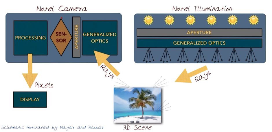
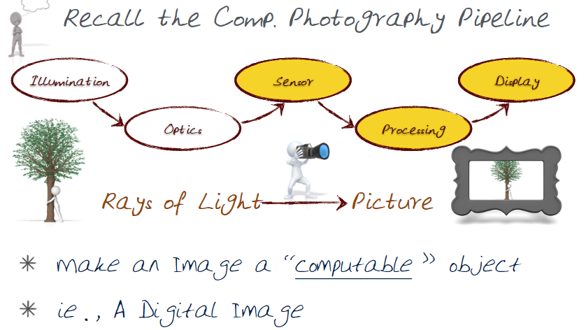
Elements of Computational Photography (Computational Photo Pipeline)

1. A scene ( Each object is effectively emitting light )
2. Source of Illumination ( The sun, a light bulb etc )
3. Optics
4. Sensor (Chemicals in the past, light sensors today)
5. Processing
6. Display ( Sharing )
7. User ( Interaction )

Dual Photography

Compuational Photography using a Dual Photograph example

Recall the Ray to Pixels "Novel Camera" example from previous section. In the next example, below, the camera is basically any type of photocell that captures light. Just replace the photocell with a camera. Here we're also presuming that we can control the aperture represented by the yellow cells.

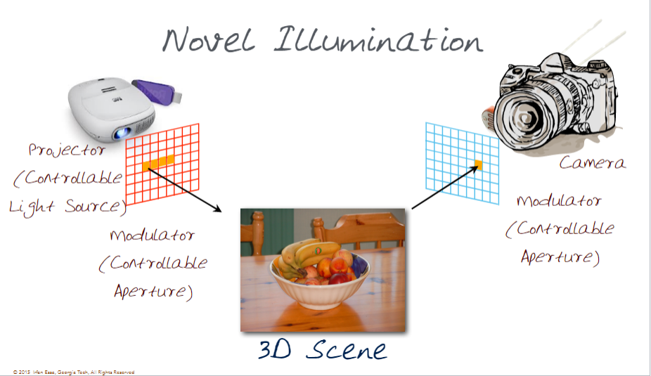
We can also relate an aperture cell to a light source cell

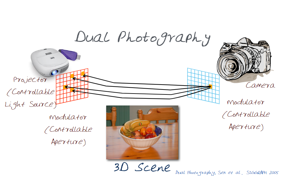
When relating from a sensor back to a cell we need to take into account the reflective properties of light. This allows us to take an image from the viewpoint of the camera. How it works: Dual photography is the process of measuring the light transported to generate the dual image. For each pixel in projector we measure the light using the sensor and store the value measured by the photo sensor as a function of pixel location. We repeat this process for each pixel in the projector. Then we use Helmholtz reciprocity, which states that the light transfer will be same along the light path regardless of the flow of light. Meaning that the same value would be measured whether the light starts off at the projector pixel and goes to the photosensor or if it starts at the photosensor and travels vice versa.

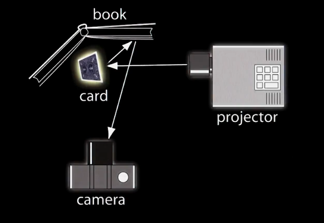
Consider the above example. How would you determine the face of the card given the POV of the camera? Well you look at the light diffused, bouncing, from the page of the book.

Panorama

Goal: To stich together a series of images together to make a single image.

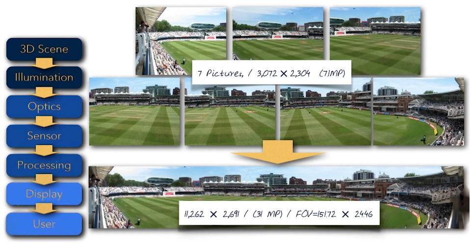
So we take a series of pictures. Ideally you'd want to fix the camera on an axis. Then align the images, blend, and merge. In order to do this there should be some commonality, or overlapping of areas. These common features can be matched to align/merge each image together.

• Step 1 - Capture the images
• Step 2 - Detection and matching
• Step 3 - Warping - adjusting the perspective in the two images to align.
• Step 4 - Fade, Blend, or Cut.
• Step 5 - Crop if necassary

Why study CompPhotography

Goal: To explore and understand the importance of computational photography.

Cameras have become more and more pervasive, smaller, and ubiquitous. There have been significant improvements in Optics. An entire field of Applied Optics has studied every aspect of lenses.

The next image illustrates the growth of various types of cameras. What isn't shown are cellphone cameras, it would diminish all the others.

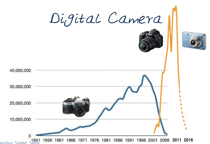
Computational Photography is about the extension of FP/DP. It uses computations to approximate the features found in dslr, and other high end, cameras.

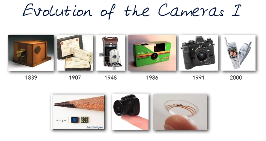
Image Processing

P2.01 Digital Images

Lesson topics:

• Digital Images - pixels and image resolution
• Discrete (matrix) and continuous function representation
• Grayscale and Color Images
• Digital Image Formats

A digital image is a matrix with a width and height. The axis begins at the top left corner (x=0=width,y=0=Height). x*y = total pixel count. A pixel is picture element that contains the light intensity at some location in the image. I(x,y) is the function that returns the intensity at a point. In a greyscale image the matrix values are quantized to be between 0 and 255.

In colour images the same principles apply but there is a 3rd dimension that represents the channel.

Raster image formats store a series of coloured dots as pixels. Images can be 16,24,32 bits per pixel. Gif, jpeg, BMP are examples of raster image formats.

OpenCV

import cv2
im = cv2.imread(PATH_TO_IMAGE_FILE)
cv2.imwrite(PATH_TO_DEST, imagename)

P2.02 Point Processes

In this section we look at how to manipulate images at the pixel level

• Point-process computations on an image

• Combining intensities from multiple images

• Add/Subtract Images

• Alpha Blending
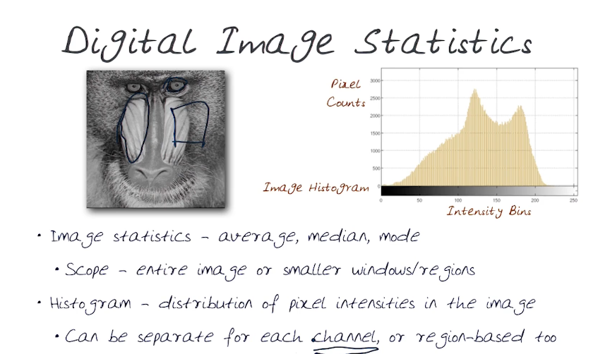
• More about image histograms

Add/Subtract : Suppose you have two images (A & B) in Matrix formats. Then A+B is simply an element wise addition, but this may lead to values outside the range (say 0-255). Similarly A-B may lead to negative values outside the range. The answer to these problems is scaling. Interestingly, subtraction is often used to spot the difference between two images. This is also often called back ground subtraction. One form of scaling is weighing so say (0.5A)-(0.5B), should produce a result within your range. One way of scaling is to take the range of the result and reduce it proportionally to the domain range of values

Alpha Blending : Along the same lines as weighting this refers to using an alpha value to introduce transparency, or opacity, into an image $\alpha RGB$

P2.03 Blending modes

Goal : How to blend two pixels from two images, for example $f_{blend}(a,b)=(a+b)/2$.

Arithmetics Blend Modes

• Division can brighten a photo
• Addition, and subtraction, gets you many white.
• Difference (subtract with scaling)
• Darken $f_{blend}(a,b)=min(a,b) over each channel$
• Lighten $f_{blend}(a,b)=max(a,b) over each channel$

• Multiply $f_{blend}(a,b)=(a*b)$ leads to darker images
• Screen $f_{blend}(a,b)=1-(1-a)(1-b)$ leads to brighter images
• Overlay
  • $f_{blend}(a,b)= 2ab$ when a < 0.5
  • $f_{blend}(a,b)= 1-2(1-a)(1-b)$ otherwise

Dodge & Burn, Dodge builds on screen mode, Burn builds on multiplication

P2.04 Smoothing

Goal: Manipulating(aka Filtering) the neighborhood of image to produce an effect such as smoothing/blurring. Another way of describing this is as an operation on a submatrix. Consider the below toy example. We have a 9x9 matrix with mostly zeros and some values equal to 90. We want to perform a simple smoothing by using an average over a 3x3 window neighborhood of a pixel. the process is pretty straight forward.

Filtering Process

For each AxA Matrix in the input(i,j)
    compute the average
    set output(i,j) = average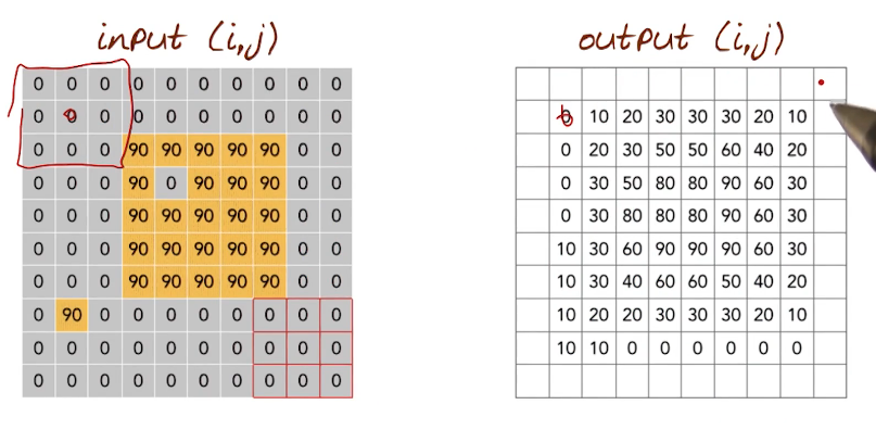

Now we are left with the missing border values, the edges. One way of doing this is to simply pad, or expand the original image and repeat the edge values

There are several popular methods for smoothing the edges: 1) Wrap around, 2) Copy edge, 3) reflect across and many others.

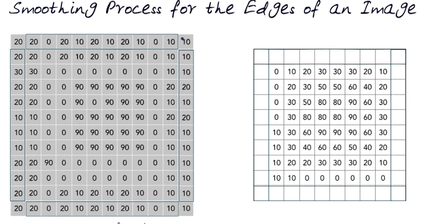
Some words on terminology. For a 3x3 area like that descibed above we say that k=1 where k is the kernal size, The window size = 2*k+1 (which yields 3 in this case) and therefore our window is 3x3.

Which can be written mathematically as
$G[i,j] = \sum_{u=-k}^k \sum_{u=-k}^k h[u,v] F[i+u,j+v]$

BOX FILTER

import cv2 

img = cv2.imread('opencv_logo.png')

# Create a 5x5 window driven by 1/25 box kernal
kernel = np.ones((5,5),np.float32)/25

# Applies the window matrix to the image
dst = cv2.filter2D(img,-1,kernel)

MEDIAN FILTERING

There is no kernal since the median is a function rather than an average.

median = cv2.medianBlur(img,5)

• reduces noise
• preserves edges and sharp lines

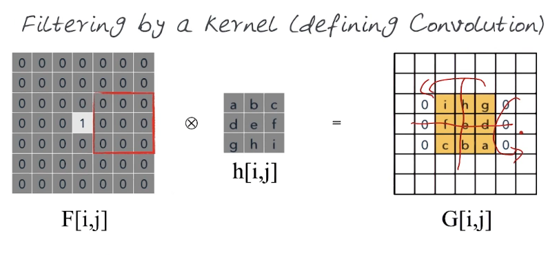
P2.05 Convolutions & Correlations

• Cross-correlation
• Convolution
• differences & properties

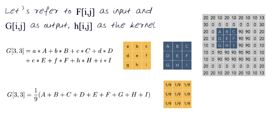
Recall our smoothing equation from the last section $G[i,j] = \sum_{u=-k}^k \sum_{u=-k}^k h[u,v] F[i+u,j+v]$. This is an example of Cross-Correlation. It's the process of applying nonuniform (h[u,v]) weights over each pixel-neighbourhood (F[i+u,j+v]) of a matrix (or image).

Definition: Cross-Correlation is a measure of similarity of two waveforms as a function of a time-lag applied to one of them. Can be thought of as a sliding dot product or sliding inner-product. Our equation can now be written as $G = h \otimes F$.

Gaussian Filter Places the greatest weight on the centre pixel and less at the edges of the kernal window. Think of it like you would a normal distribution centred at the mean weight over the centre pixel.

Convolution is similar to the Cross-Correlation. What happens if we flip the Cross-Correlation equation $G = h \otimes F$, ie $F \otimes h = G$. Look at what happens when we use an impulse function/matrix (left) and apply it to the h kernel. We get an inverted and flipped, or translated, h as a result.

1. Cross-Correlation
   $G[i,j] = \sum_{u=-k}^k \sum_{u=-k}^k h[u,v] F[i+u,j+v]$ Denoted $G = h \otimes F$
   NB_1 Any image cross correlated with a gaussian filter will have a Blurred output NB_2 An impulse image Crossed with a Gaussian Filter will have an Blurred output

2. Convolution
   $G[i,j] = \sum_{u=-k}^k \sum_{u=-k}^k h[u,v] F[i-u,j-v]$ Denoted $G = h \ast F$
   NB_1 Any image convolved with a Box filter will have an averaged output NB_2 An impulse image convolved with a box filter will have an Averaged Output

Cross-Convolution and Convolution produce the same result when the kernel used is symetric in both X and Y

Convolution Properties

• Linear and shift invariant - ie it behaves the same everywhere. The output depends on the pattern in the image neighbourhood and not the position of the neighbourhood
• Commutative $ F \ast G = G \ast F$
• Associative $ (F \ast G) \ast H = F \ast (G \ast H) $
• Identity is the Unit Impulse $E = [\dots,0,0,1,0,0,\dots ]$
• Seperable - if the filter is seperable as well then we can convolve all rows, then convolve all columns

P2.06 Gradients

Detecting features in an image, in particular edge detection using image gradients (discrete & continuous)

Recall Cross-Correlation and convolution from our previous section. How can we use these operations to find features and which filters should we use? Suppose we want to align two images. Our first step would be to detect common features that have a correspondance to the other image. Of course some features will be easier than others. In particular edges, and other discontinuities, can be a beneficial feature.

Discontinuities

• Surface Normal - exist where there is a shape whose edges drop quickly
• Depth - occur when there are overlapping shapes
• Surface Colour - differences in colour
• illumination - lighting/shadows reveal changes

Edge Detection
Look for neighbourhood, a window?, with a strong sign of change, ie pixel values change rapidly along one or more axes. The neighbourhood size will be defined as k. We will also need to define how we define the sign of change, a threshold.

Let's define an edge as an area where there is a rapid change in the image intensity function

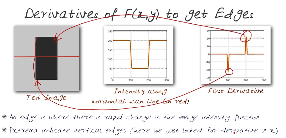
The idea is rather straight forward. To implement we need an operation that when applied to an image returns it's derivatives. How we do this is by creating masks/kernels that when applied return the image gradient. Then we apply the threshold to select edge pixels, this is done using the convolution operator.

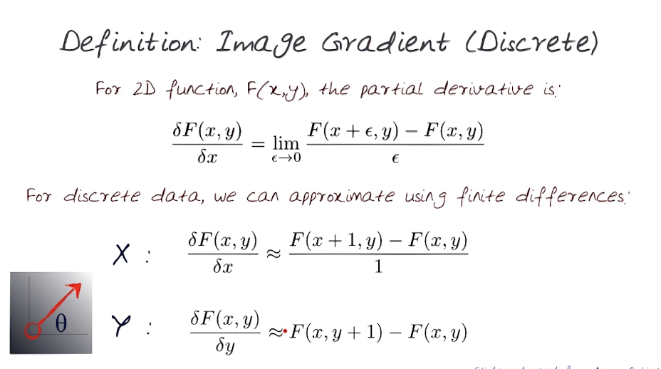
Differential Operators for images
Define:
Gradient of an image is a measure of change in the Image Function F in x and y. $\triangledown F = [ \frac{\partial F}{\partial x},\frac{\partial F}{\partial y} ]$
Holding y constant at 0 we can compute the first term, and holding x = 0 we compute the second term.
We can build on this to compute the gradient direction (aka angle) as $\theta = tan^{-1} [ \frac{\partial F}{\partial y} / \frac{\partial F}{\partial x} ]$
Additionally we can compute the Gradient magnitude as the strength of the edge $|| \triangledown F || = \sqrt{ (\frac{\partial F}{\partial x})^2 + (\frac{\partial F}{\partial y})^2 }$

P2.07 Edges

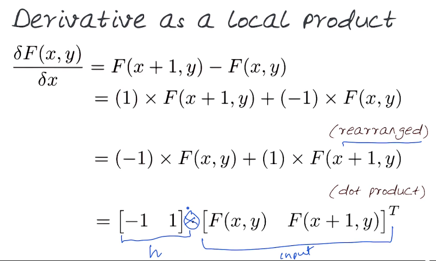
To apply this to a discrete matrix, such as an image, we need a mask/kernel that effectively computes a discrete values using cross-correlation (ie finite differences). (Recall that finite differences provide a numerical solution for differential equations using approximation of derivatives).

Here are a couple of examples, note that these are not symmetric about a point

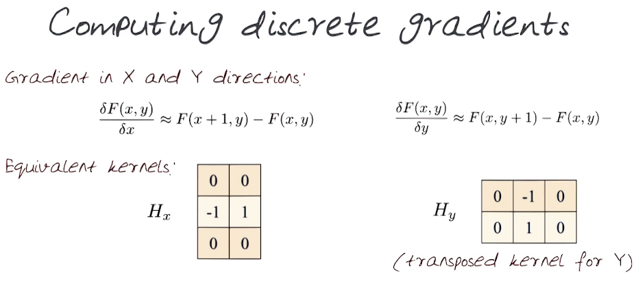
Here are some more popular ones

X-direction       Y-Direction
 0   0   0        0  1/2  0
1/2  0  1/2       0   0   0
 0   0   0        0  1/2  0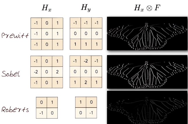

Now that we know how to compute the gradient. How do we use this to detect edges.

Recall, Convolution is $G = h \ast F$ and the derivative of a convolution is $\frac{\partial G}{\partial x} = \frac{\partial}{\partial x}(h \ast F)$. If D is the kernel used to compute derivatives, and H is the kernel for smoothing. Then we could define kernels with the derivative and smoothing in one: $(D \ast H) \ast F$

Gradients to edges

1. Apply smoothing to suppress noise
2. Compute the gradient
3. Apply edge enhancement - enhance the lines representing the gradients
4. Edge localization (enhance and differentiate edges from noises)
5. Threshold and thinning

Canny Edge Detector

• Filter image with the derivative of a Gaussian
• Find the magnitude and oritentation of the gradients
• Non-maximum suppression
  • Thin multi-pixel wide ridges down to a single pixel width
• Linking and thresholding (hysteresis)
  • Define a high and low threshold
  • Use the high threshold to start an edge curve and the low threshold to continue them

Cameras

P3.01 Camera

Cameras: Pinhole cameras and optics

Objectives:

• Rays to pixels
• Camera without optics
• Camera lens system
• The lens equation

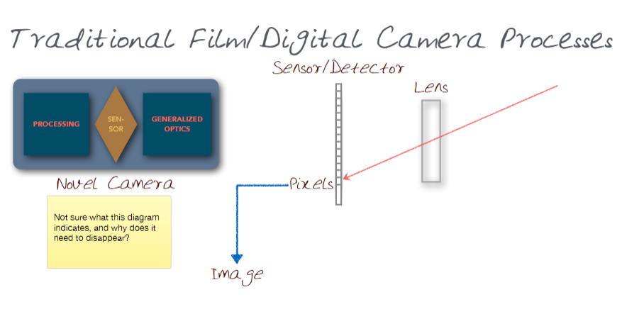
Previously we've spoken about the computational photography pipeline on a ray of light. When we take a photo we are capturing the light, the geometry, and the scattering of light.

How can we build a camera without optics? Pretty simple: Just think of a pinhole camera or camera obscura. As it turns out you don't need a lens to create an image. But you do need to restrict the light rays.

Pinhole Camera Characteristics:

• No distortion: straight Lines remain straight
• Infinite depth of field: Everything in focus (there may be optical blurring)

The size of the pinhole, the aperture, is a constraint on the amount of light. The larger the aperture the more light is let into the image. to the point that the image becomes blurred when it's too large. A smaller aperture means more diffraction.

For pinhole diameter d and a distance from pinhole to sensor f and the wavelength of light $\pi$
$d = 2 \sqrt{\frac{1}{2} f \pi}$

Now we want to replace the pinhole with a lens: Parallel rays will still converge to the focal length f.

Lens Equation
$\Large \frac{1}{o} + \frac{1}{i} = \frac{1}{f}$

Where o is the length from the object to the lens, i is the length from the image to the lens.

P3.02 Lenses

P3.03 Exposure

P3.04 Sensor

Transformations

P4.01 Fourier Transforms

• using sines and cosines to reconstruct an image
• the fourier transform
• Frequency Domains for a signal
• three properties of convolution relating to Fourier Transforms

Basic Building Block
$f(t) = A cos(n \omega t)$ where A=Amplitude, and $\omega$ is the frequency

Here you can see multiple scenario for n = 1,2,3,4

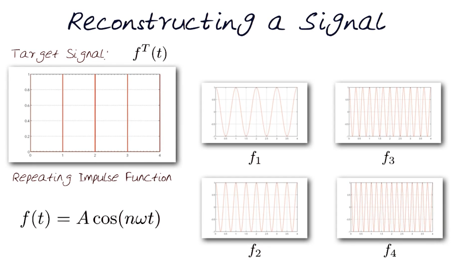
These can also be summed together to form an even greater number of models.

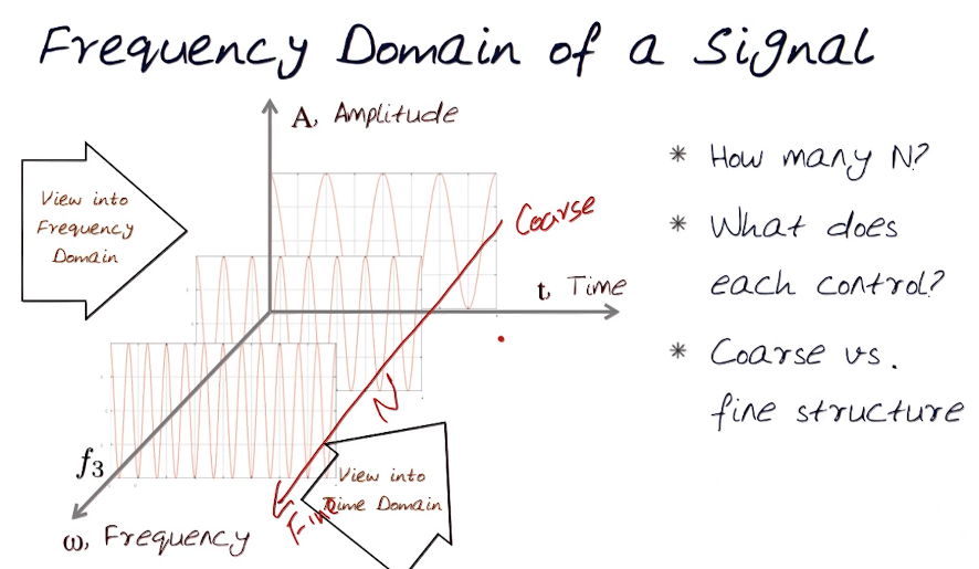
Fourier Transforms:

• A periodic function can be expressed as the weighted sum of sines and cosins of different frequencies
• Transforms f(t) into $F(\omega)$
• Frequency spectrum of the function f
• A reversible operation
• For every omega from 0 to infiinty $F(\omega)$ holds the amplitude A and phase $\phi$ of a sine function $F(\omega) = A cos(\omega t + \phi)$

We can use these frequencies to create approximations. For example $A = \sum_{1}^{\infty} \frac{1}{k}sin(2 \pi k t)$ can have the same effect as a box filter

Convolutions & Fouriers

1. Fourier transform of a convolution of two functions is the product of their respective fourier transforms
   • $F[g \ast h] = F[g] \ast F[h]$
2. Inverse Fourier transform of the product of two fourier transforms is the convlution of the two inverse fourier transforms
   • $F^{-1}[g h] = F^{-1}[g] \ast F^{-1}[h]$

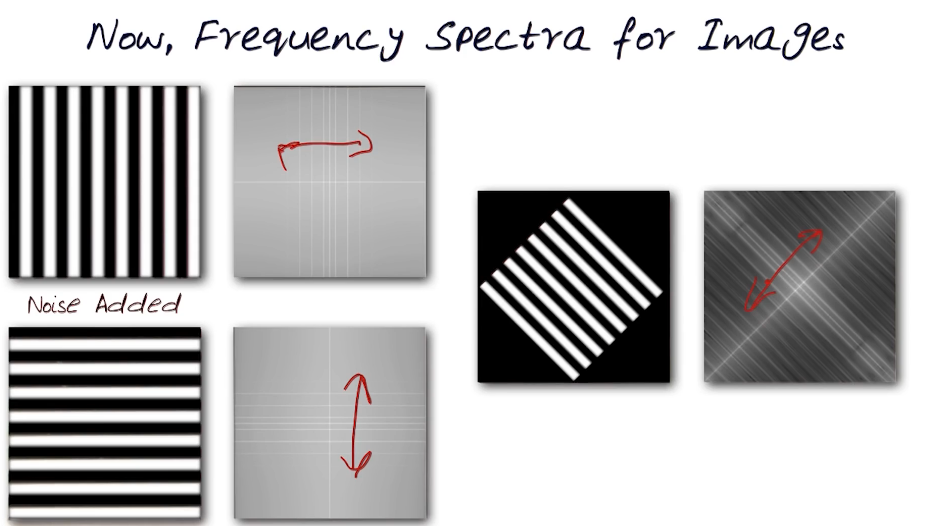
Of course the above are highly constructed for the purposes of illustration. A real image will have a much messier frequency spectra.

Recall that

• "For every omega from 0 to infiinty $F(\omega)$ holds the amplitude A and phase $\phi$ of a sine function".
• It uses Real and complex numbers to achieve this
  • $A sin(\omega t + \phi)$
  • $F(\omega) = R(\omega) + j I(\omega) $
  • $A \pm \sqrt{R(\omega)^2 + I(\omega)^2}$
  • $\phi = tan^{-1} \frac{I(\omega)}{R(\omega)} $

Blurring and Frequencies: we can apply a box or gaussian filter, then subtract to produce a line/edge image

P4.02 Blending

How can we blend multiple images by applying our learning so far?

• merging two images
• Window sizes for merging images
• Advantages of using the fourier domain in blending

Recall: Combine, Merge, Blend images
Our goal is two create one smooth image from multiple images. A basic approach might be to take 50% of each pixel values and add them together to get a final result, overlapping the two.

A second approach might be to take the first half of image one and the second half of image two and place them side by side. In this approach we would be left with a sharp difference in the final image that we need to get rid of. to handle this we introduce the idea of Cross-Fading. What we do here is create a ramp of weights. For the left image we go from 1 to 0 as we move from left to right, for image two we go from 0 to one. Consider what will happen here. As we near the border area the weight shift from image one to image two. The blending area is referred to as the blending window, we don't perform blending outside this window.

It should be noted that the window size here will have a significant effect on the resulting image. the smaller the window the crisper, or more distinct the blend.

What's the optimal window size?

• To avoid seams: Window = Size of the largest prominent feature
• To avoid ghosting: Window <= 2xSize of smallest prominent feature

Using Fourier Domain this means

• Largest freq <= 2* size of smallest frequency
• Image freq content should aoccupy one octave (power of 2)

Method:
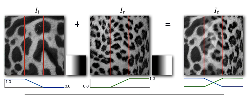
Suppose we have two images, a left and a right, and we label them $I_l$ and $I_r$
Let FFT => Fast Fourier Transform

• Compute $FFT(I_l)=F_l$ and $FFT(I_r)=F_r$
• Decompose Fourier image into octaves (Bands)
  • $F_l = F_l^1 + F_l^2 + F_l^3 + ...$
  • $F_r = F_r^1 + F_r^2 + F_r^3 + ...$
• Feather corresponding octaves of $F_l,F_r$
• Compute inverse FFT and feather in the spatial domain
• sum feathered actaves images in frequency domain

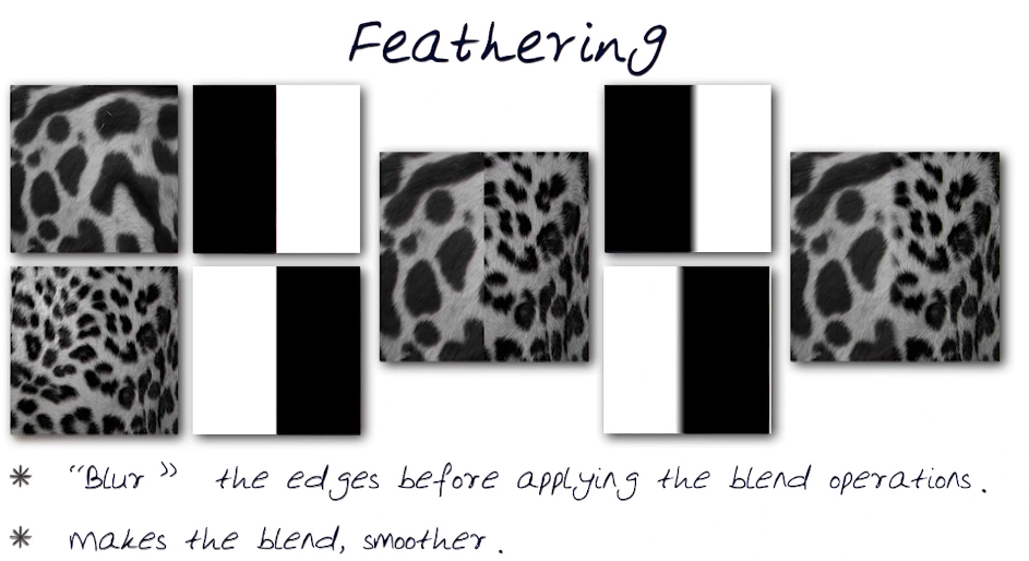
What is Feathering?

P4.03 Pyramids

Objectives

• Gaussian and Laplacian pyramids
• Use of Pyramids to encode the freq domain
• Compute a Laplacian Pyramid from a Gaussian pyramid
• Blend two images using pyramids

Recall: Optimal Window size & Fourier Domains from previous section

Pyramid Representation
Image you have an 8x8 image, and you run a 3x3 gaussian filter over it, in doing so you want to decrease the image to a 4x4 image. You repeat the process on the 4x4 to get a 2x2 image, and again on the 2x2 to get a 1x1. This series is the pyramid. Level 0 is the original image

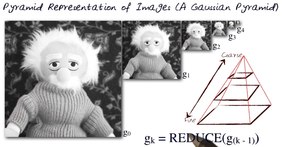
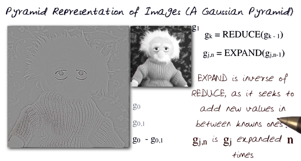
What you see in the second slide is basically an error image and is referred to as the Laplacian. Each laplacian level is simply the error or difference between two consecutive levels in the gaussian pyramid.

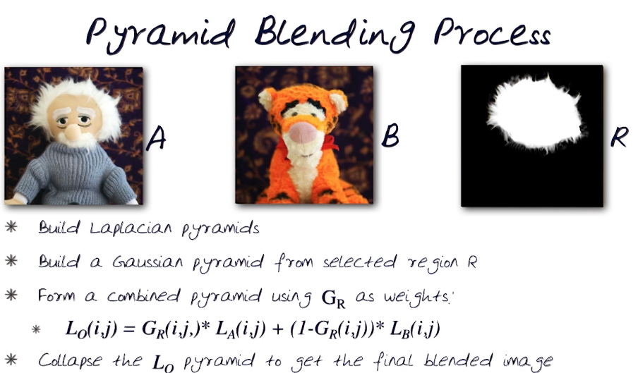
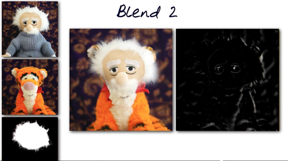
Blending Step Suppose you have two images, a left and a right.

• For each image compute the gaussian, and laplacian, pyramid
• begin the blending by merging each image at each level and working from coarse to fine

P4.04 Cuts

Objectives:

• Additional Method merging images
• Finding seams in images
• Pros of cutting vs blending

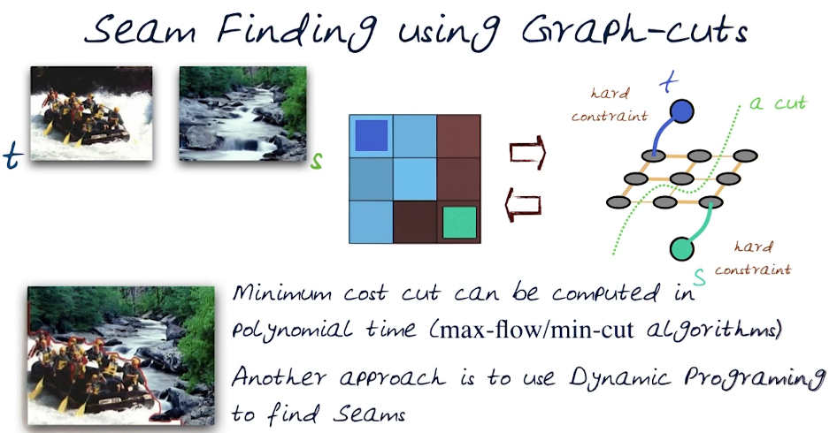
The idea here is similar to a side by side placement of the two images. However, we use a non-straight boundary rather than a straight x or y line. By doing this in a nonstraight cut we can match features in each image that may not lie in a straight line. Note that this may still lead to ghosting which we will need to address. We need to find an optimal seam to integrate the two images.

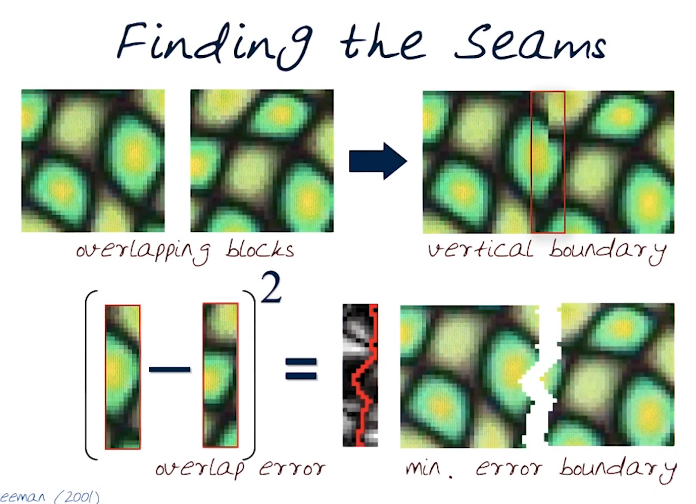
When we put the last two images together the result will be virtually seamless!

This method can also be used to extend an image, by repeated merging of certain areas in a cut

How it's done, Assume we have a target(t) and source(s) image

• We create a matrix representation of the result ( a blank slate )
• Next we create a node structure
  • for each node we need a cost function
  • this represents how strong the bond is to each neighbouring pixel
  • some are bonded heavily to the target image and others to the source image
• the final result will be an image driven where the decision is determined by the cost function

P4.05 Features

Objectives:

• Benefits of using feature detection
• What makes good features
• Harris Corner detection
• SIFT detector

Recall our discussion about feature detection and matching across multiple images. The matching pipeline now depends on locating similar features in multiple images.

Basics of image matching: Suppose the image is viewed in the context of a larger xy-axes. These are not the image axes but rather an x & y that contains the image as well as possibly it's transformations.

It's should be intuitive to see that a feature in the original image will still exist in the transformed image, albeit in an altered state. We want to find these similar points precisely and reliably and localized. However, we don't always get what we want.

Characteristics of good features:

• Repeatability/Precision - regardless of slight transformation
• Saliency/Matchability - there needs to be characteristics that make them matchable
• Compact/Efficient - need to be easy to compute
• locality - features should be contained in a relatively small area in the image

In a nutshell the more distinctive, or unique, a small area is the better it will be as a feature. Corners are one good feature, as are objects. An area with a single colour would be difficult to detect.

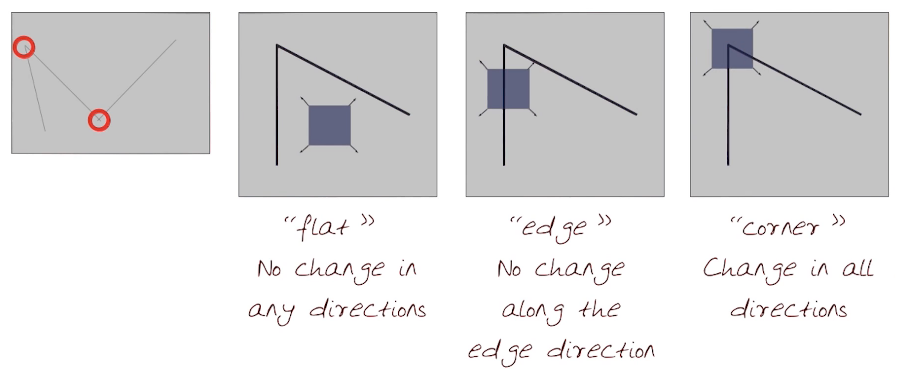
Corners are repeatable and distinctive features, with the property that in their local region the gradient will have 2 or more dominant directions. One gradient is horizontal, the other will be vertical. We can recognize a corner point by looking through a small window. Shifting the window in any direction causes a large change in intensity due to the corner gradient. This large change is our detection flag.

In the following image the grey square represents our viewing window.

The math

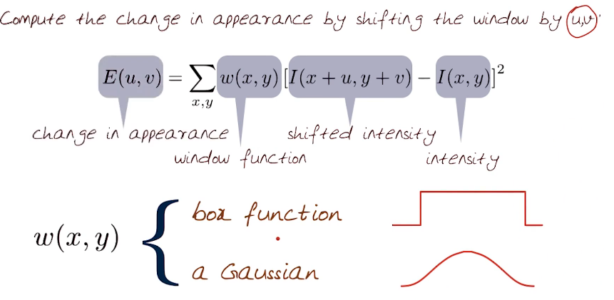
We compute the change by measuring the appearance caused by shifting the window u,v pixels.
$E(u,v) = \sum_{x,y} w(x,y)[I(x+u,y+v)-I(x,y)]^2$
for some weighting function (such as a box function or gaussian)

We now proceed by using a taylor expansion to approximate $E(u,v)$
$E(u,v) \approx \begin{bmatrix} u & v \end{bmatrix} M \begin{bmatrix} u \\ v \end{bmatrix}$
Where M is the second moment matrix computed from the Image derivatives/gradients $I_x$ and $I_y$
$M = \sum_{x,y} w(x,y) \begin{bmatrix} I_x^2 & I_x I_y \\ I_x I_y & I_y^2 \end{bmatrix}$
When we put this M matrix back into $E(u,v)$ we get a rather nice result
$E(u,v) = \sum_{x,y} w(x,y)[u^2 I_x^2 + 2uv I_x I_y + v^2 I_y^2 ] $
The second term on the right tells us that the surface change in appearance can be locally approximated by a quadratic form, or window. This quadratic is a slice of an ellipse on a window. For eaxample $[u^2 I_x^2 + 2uv I_x I_y + v^2 I_y^2]=k$ would define an elipse on a window of size k.

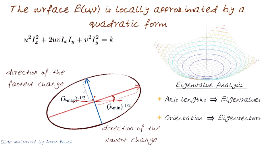
Recall that $[u^2 I_x^2 + 2uv I_x I_y + v^2 I_y^2]=k$ is simply $\begin{bmatrix} u & v \end{bmatrix} M \begin{bmatrix} u \\ v \end{bmatrix} = k$
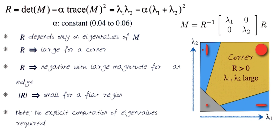
So ... This tells us that M is a diagonal matrix that can also be written as $ M = R^{-1} \begin{bmatrix} \lambda_1 & 0 \\ 0 & \lambda_2 \end{bmatrix} R$
where the lambdas represent our eigenvalues and $R = det(M) - \alpha trace(M)^2 = \lambda_1 \lambda_2 - \alpha(\lambda_1 + \lambda_2) $
This R is the key to detecting corners.

• R depends only on the eigenvalues of M
• R is large for a corner
• R is a large negative value for an edge
• |R| is small for flat regions

P4.051 Harris Detection Algo - Preview

Preview - will be discussed in depth later

• Compute gaussian derivative at each pixel
• Compute second moment matrix M in a gaussion window around each pixel
• Compute corner response function R
• Threshold R
• Find local maxima of response function (Non-maximum suppression)

Properties of a Good Harris detectors

• Rotation Invariant
  • Elipses rotate but the shape & eigenvalues remain the same
  • Corner response R is invariant
• Intesity Invariant
  • not affected by the intensity of the image
  • partial invariance to additive and multiplicative intensity change
• Scale Invariant?
  • No - It depends heavily on the size and scale of the window size
  • Using pyramids or frequency domain is one option for overcoming this

P4.06 Features Detection/Matching

Objectives:

• Deeper dive into the Harris corner detector
• Deeper dive into the SIFT algorithm
• How Harris & SIFT work

Harris Detector

• Compute Horizontal & vertical derivatives of the image
• Compute outer products of gradients M
• Convolve with larger Gaussian
• Compute scalar interest measure R
• Find local maxima above some threshold, detect features

Algorithm

• Compute gaussian derivative at each pixel
• Compute second moment matrix M in a gaussion window around each pixel
• Compute corner response function R
• Threshold R
• Find local maxima of response function (Non-maximum suppression)

Properties

1. Invariant to Rotation - Yes
   Ellipse rotates but it's shape remains the same (ie eigenvalues don't change)
   Corner response R is invariant to image rotation
2. Invariant to Intensity - Yes Generally invariant to additive and multiplicative intensity changes Only derivatives are used (adding,multiplying by a constant doesn't change the derivative)
3. Invariant to Scale - No A corner in a small image may appear as an edge in an enlarged image

In order to overcome the 3rd point the region/window needs to change as well. How to we figure out how to change it? How do we choose corresponding regions. The general method is to choose the scale of the best corner. Basically this comes down to computing a region, circle, which is scale invariant. It should not be affected by the size and will be the same for corresponding regions. Note that The average intensity for corresponding regions, even of different sizes, will be the same.

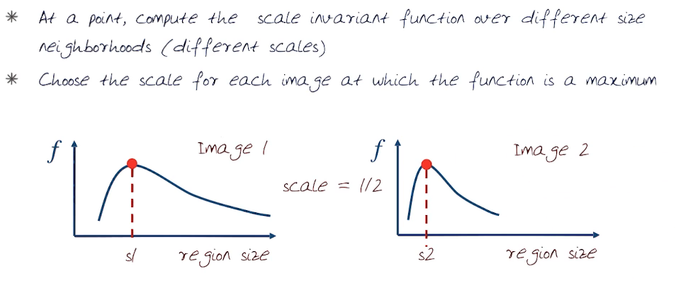
A good function for scale detection has one stable peak. For most general images a good function would be one which responds to contrast ( a sharp local intensity change ). To do this we need to find a robust extremum (a max or min) both in space and in scale. This can be done via pyramids

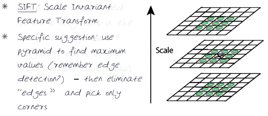
SIFT - Scale Invariant Feature Transform

Harris-Laplacian

• Find the local max of
  • A Harris corner detector in space (image coordinates)
  • A Laplacian in scale (pyramid levels)

Run a corner detector on the image (this is in space). Then look for these features at different levels of a Laplacian Pyramid.

SIFT Lowe, 2004

• Find the local maximum
  • Difference of Gaussians (DOGs) in space and Scale
  • where DOG is simply a pyramid of the difference of Gaussians within each octave

How it's done

• Orientation assignment
  • Compute the best orientation for each keypoint region
• Keypoint description
  • Use local image gradients at selected scale and rotation to describe each keypoint region

The key to SIFT is that image content will be transformed into local feature coordinates that are invariant to translation, rotation, scale, and other imaging parameters.

Image Transformations

P5.01 Intro

Objectives

• Transforming the image
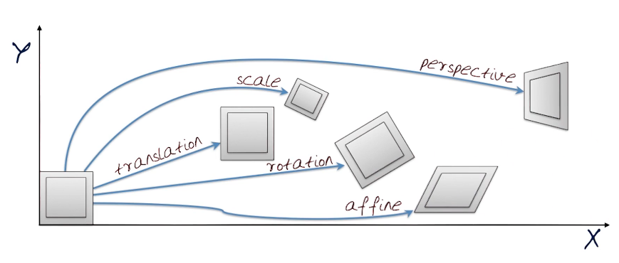
• Rigid Transformations: Translations & Rotations
• Affine/Projective Transformations
• Degrees of freedom for different transformations

How do we actually transform an image? Previously we've looked at simple transformations like blurring and sharpening. When filtering an image, like lightening, we've changed the range of values. When changing the scale, or size, of the image we change the domain of the image but not the range.

Parametric Global Warping: Change of size, scale, angle.
Let $p'$ be the new point and $p$ be the old point, then we need to find a single function T such that $p' = T(p)$. This T must be the same for any point p, and should depend on the least number of parameters. As a matrix transform T can also be written as $p' = M p$

2D Transformations

• Scaling: Multiply each component by a scalar
  • Uniform scaling: the scalar is constant in both x and y axes
  • NonUniform: scalar will be different

Consider:
$M = \begin{bmatrix} s_x & 0 \\ 0 & s_y \end{bmatrix}$ - Scale around (0,0)
$M = \begin{bmatrix} -1 & 0 \\ 0 & -1 \end{bmatrix}$ - Mirror over (0,0)
$M = \begin{bmatrix} 1 & sh_x \\ sh_y & 1 \end{bmatrix}$ - shear (parralellogram)
$M = \begin{bmatrix} cos(\theta) & -sin(\theta) \\ sin(\theta) & cos(\theta) \end{bmatrix}$ - Rotation of $\theta$

2D Translations
Consider: $x' = x + t_x$ and $y' = y + t_y$ which cannot be expressed using a simple matrix M like before. What we can do though is change to a homogenous coordinates system, by adding a 3rd coordinate to every 2d point. So (x,y) becomes (x,y,w) where w is anything but 0.

We can now consider, remodel, the previous tranformations in this new format
Recall that we want an equation of the format $p' = M p$

Translation becomes
$M = \begin{bmatrix} 1 & 0 & t_x \\ 0 & 1 & t_y \\ 0 & 0 & 1 \end{bmatrix}$

Scaling becomes
$M = \begin{bmatrix} s_x & 0 & 0 \\ 0 & s_y & 0 \\ 0 & 0 & 1 \end{bmatrix}$

As you may have noticed this can be simplified to the following

$\begin{bmatrix} x' \\ y' \\ w' \end{bmatrix} = \begin{bmatrix} a & b & c \\ d & e & f \\ g & h & i \end{bmatrix} \begin{bmatrix} x \\ y \\ w \end{bmatrix}$
So to define a transformation we need to determine the appropriate values for a,b,c,etc

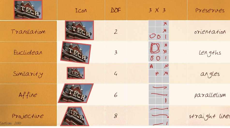
Affine Transformations (Parallelogram Effect) - 6 degrees of freedom, g=h=0, i = 1
$\begin{bmatrix} a & b & c \\ d & e & f \\ 0 & 0 & 1 \end{bmatrix}$

Projective Transform (Affine + Warp) - 8 degrees of freedom, i = 1

• Origin needs not map to origin
• Lines map to lines
• Parallel lines do not remain parallel
• ratios not preserved

Recovering Transforms? Given two images f(x,y), g(x',y'), how do we recover the transform T(x,y)? How many corresponding points do we need to know? What's happening here is we are trying to determine the matrix M.

P5-02 Image Warping

• Image Warping (Forward and Inverse)
• Warping using a mesh
• Image warping
• Feature based image warping

Recall: Image filtering changes the range of the image while warping chnages the domain of the image. In a transformation lines remain lines, but in a warping points are mapped to points. So far we have only talked about warpping we will now formalize the definition.

Let's consider two images: A source (S) and a target (T). For s we use the pixels (u,v) and for t we use (x,y).
Then

• Forward Warp can be stated as $(x,y) = [X(u,v),Y(u,v)]$
• Inverse Warp can be stated as $(u,v) = [U(x,y),V(x,y)]$

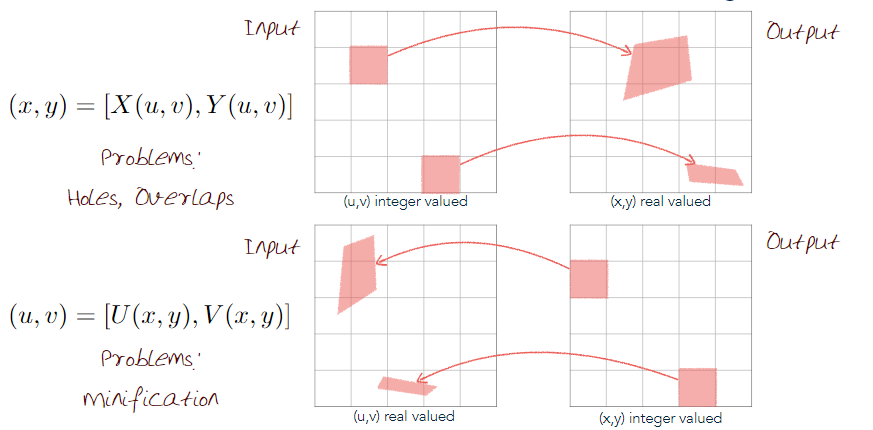
What may not be so obvious from the above image is the problem of Magnification and Minification, which arises when the value of a single pixel needs to be magnified or minified. Magnification can be resolved by distributing the colour of a pixel amongst it's neighbours (common technique for this is splatting). In a similar vein minification can be resolved by interpolating the color value from the neighbouring pixels

Mesh-Based Warping

• Use a sparse set of corresponding points and interpolate with a displacement field
• Triangulate the set of points on Source
• Use an affine model on each triangle
• Triangulate target with displaced points
• then use inverse mapping

Feature Based Image Morphing: Animations that change (or morphs) one image or shape into another through a seamless transition.

P5-03 Panoramas

Objectives:

• Generate a panorama
• Image Re-projection
• Homography from a pair of images
• Computing outliers and inliers
• Methods/Details for panorama construction

Recall: 5 Basic steps for panorama construction

1. Capture Images
2. Detection and matching
3. Warping and Alignment of Images
4. Blending,fading,Cutting
5. Cropping (when needed)

A bundle of rays contains all views, but a camera at fixed points has a limited capture of light. Each capture contains a subset bundle of the larger bundle. Can we create a synthetic view, (bundle) from the camera capture? Turns out that it is possible to create any synthetic camera view as long as it has the same centre of projection.

Image Re-Projection
To relate two images from the same camera centre and map pixels from image 1 to 2

1. Cast a ray throught each pixel in Image 1
2. Draw the pixel where that ray intersects Image 2

Think of this as a 2D warp of image 1 to image 2. The alternative approach, much more difficult, is see this as a 3D problem. We will determine the warp by using/computing a Homography.

Homography is a way to relate two images with the same camera centre.

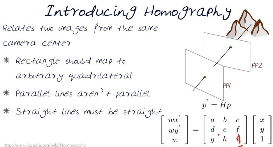
Let's look at how to compute this. The process builds upon our discussion in the previous section regarding warping. First we need to find a common feature in both images. We can then determine the four points that draw a bounding box around the feature. Then we can solve for the M matrix.

Mathematically:
Recall the equation $p' = Mp$ where $p$ and $p'$ are corresponding points from each image
Let $p_1 = (x,y)$ and $p'_1 = (x',y')$ where $(x',y') = (wx'/w, wy'/w)$
NB For this type of problem we replace M with H

$\begin{bmatrix} wx' \\ wy' \\ w \end{bmatrix}

\begin{bmatrix} a & b & c \\ d & e & f \\ g & h & 1 \end{bmatrix}\begin{bmatrix} x \\ y \\ 1 \end{bmatrix}

$ Now set up a system of linear equation $Ah = b$ where h is our vector of unknowns $h=[a,b,c,d,e,f,g,h]^T$ Finally we can solve for h using a least squares solution $min||Ah - b ||^2$

Bad matches, How to handle? For this we use a RANSAC, Random Sample Consensus. Which is a form of voting alogrithm. We will take one match between the two images, count the number of inliers, and compute the average translation vector.

RANSAC
Loop to find a convergence to a popular H:

• randomly select 4 feature points
• compute homography matrix H
• compute inliers where $SSD(p'_{in}, Hp_{in}) \lt \epsilon$
• keep largest set of inliers
• recompute least-squares H estimate on all of the inliers

The idea here is not that there are more inliers than outliers. It is that the outliers are wrong in different ways

Handy Functions in doing this

# Read in your images

#Initialize your feature detector (SIFT)
orb = cv2.ORB()

# Find your keypoints
kp1,des1 = orb.detectAndCompute(img1,None)
kp2,des2 = orb.detectAndCompute(img2,None)

# Draw your keypoints ...

# Match them
bf = cv2.BFMatcher(cv2.NORM_HAMMING,crossCheck=True)
matches = bf.match(des1,des2)

# At this point you'll want to create lists of keypoints for each of the matches

# Get the homography
MHom,inliers = cv2.findHomography(pts2,pts1,cv2.RANSAC)

# Create your panorama now ... numpy is great here
imgPanorama = cv2.warpPerspective(img2,MHom,panaromaSize)

# etc etc

Final thoughts: In our discussion we talk about a sequence of images where we take the pictures in the same order we stich them. This is not actually necassary though. Using the RANSAC algorithm the order in which the pictures are taken or given is no longer necassary, so long as the existence of the features is there.

P5.04 High dynamic Range

Objectives:

1. Dynamic Range
2. Digital cameras do not encode dynamic range very well
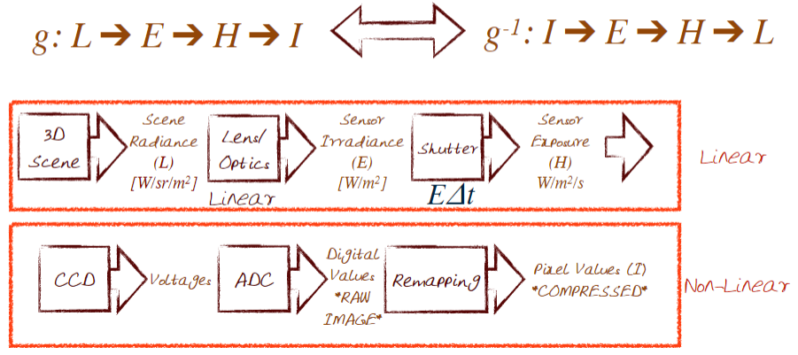
3. Image Acquisition pipeline for capturing scene radiance ot pixel values
4. Linear and non-linear aspects inherent in the Image acquisition pipeline
5. Camera calibration - to get the right levels that can be replicated
6. Pixel values from different exposure Images will be used to render a radiance map of a scene
7. Tone mapping

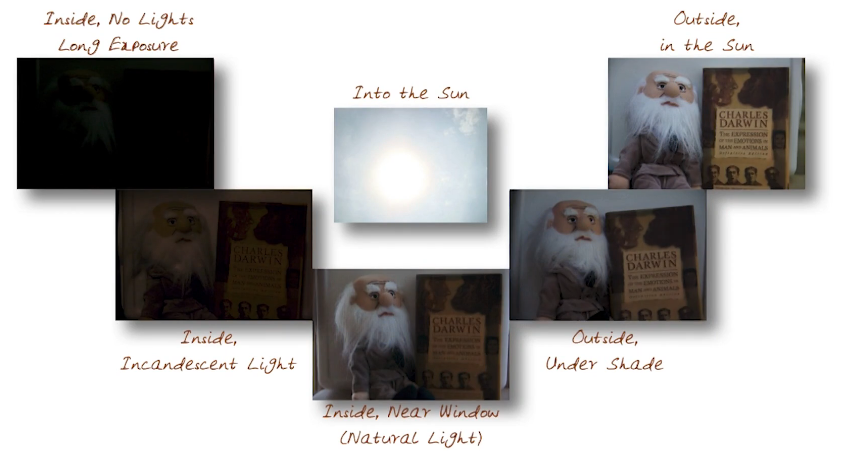
An example of dynamic Range in the real world.

Luminance: A photometric measure of the luminous intensity per unit area of light traveling in a given direction measured in candela per square meter (cd/m^2).

• Human Contrast Ration (static) is about 100:1 or 10^2 => about 6.5 f-stops
• Human Contrast Ration (dynamic) is about 1,000,000:1 or 10^6 => about 20 f-stops

The difference between dynamic and static here simply refers to whether or not the light is changing. For example a short exposure often leads to under-exposed images at the upper end of the high dynamic range. Similarly a long exposure can lead to an over-exposed image where the lower end of the dynamic range is packed into values from 0 to 255. ($W/sr/m^2$) is Watts per steridian metre squared.

Most current camera's have a limited dynamic range. Image you have two images of the same scene, the difference between the two is the length of exposure. In order to capture the dynamic range of both images you would need 5-10 million values. But an 8-bit images only contains 256 values.

Let's re-examine the relationship between Image and Scene Brightness (Image acquisition pipeline)

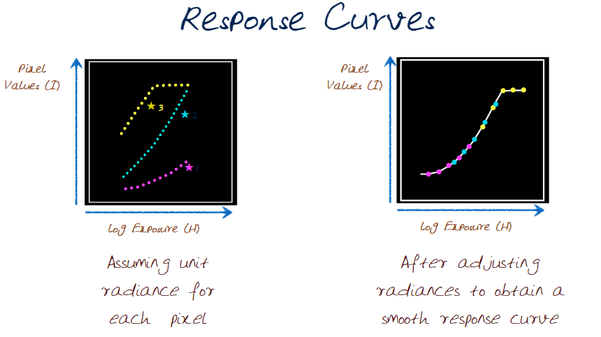
Performing a radiometric calibration requires a colour chart with known reflectances, and multiple camera exposures to fill up a response curve. We want to do is be able to take several images at different exposure levels and create a stack of sorts. Why we do this is to create a radiance response curve.

Note that for a series of images with exposures $\Delta t = {1/64, 1/16, 1/4, 1, 4}$ (Measured in seconds)
Pixel_Values(I) = g(Exposure)
Exposure(H) = Irradiance(E) * $\Delta t$
Log Exposure(H) = log Irradiance(E) + log$\Delta t$

How this works is you take a few points and measure the same points value (at each exposure level) to get Pixel_Values(I). What you see in the left image is the plot for each of three points. Each colour here represents a point or feature. The result is a response curve. The image on the right side is what we want. We will need to manipulate our intensities to get this.

To compute this?

• let $E_i$ be the exposure of the pixel site $i$
• let g(z) be the discrete inverse response function
• for each pixel site i in each image j compute
  • $ln(E_i)+ln(\Delta t_j) = g(Z_{ij})$
• Now solve the overdetermined linear system for N pixels over P different exposure images
  • $\sum_i^N \sum_j^P [ln(E_i)+ln(\Delta t_j) - g(Z_{ij}) ]^2 + \lambda \sum_{z=Z_{min}}^{Z_{max}} g''(z)^2$
  • can be solved using a linear least square approach

The first part is the fitteng term and the second part is the smoothness term.

Using this we can create a curve for each colour and then we use these curves to create a radiance map. But these require a special type of file format of which there are several out there.

Let's take a quick look at the RGBE 4 channel format:
Examples: (145,215,87,149) = (145,215,87) 2^(149-128) = (1190000,1760000,713000)
(145,215,87,103) = (145,215,87) 2^(103-128) = (0.00000432,0.00000641,0.00000259)
Note that 128 is simply the ceiling of 255/2, and 255 is simply the max value in 8-bits of information

Tone Mapping Many well known algorithms exist for this.

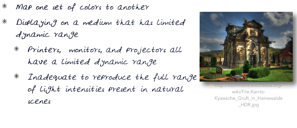
On the other hand we have Tone Mapping which seeks to address the problem of a strong contrast reduction from the scene radiance to the displyable range while preserving the image details, colour, and appearance. Notice the ghosting in the image above. This is a common problem in tone mapping which tries to pack the entire high dynamic range into 0 to 255.

P5.05 Stereo

Stereo images: Multiple viewpoints of the same scene

Objectives:

1. Geometry (Depth Structure) in a scene
2. Stereo
3. Parallax
4. Compute Depth from a stereo image pair

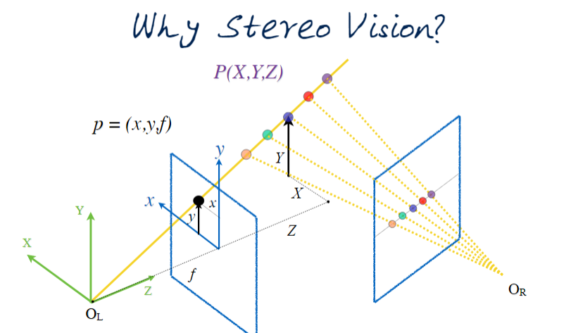
Review depth of a scene (below) in geometric terms.

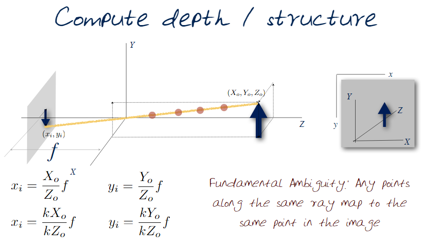
Here $(x_i,y_i)$ represent the captured image, and $(X_0,Y_0,Z_0)$ represent some object. It should be noted that there is a fundamental ambiguity that may not be so obvious here: The equations don't change. For any point along the yellow line the equations are the same and only the values change. This means that we can scale any of the co-ordinates along the line with a constant. To help resolve this ambiguity we introduce the idea of stereo vision. Which is the use of multiple viewpoints to understand depth.

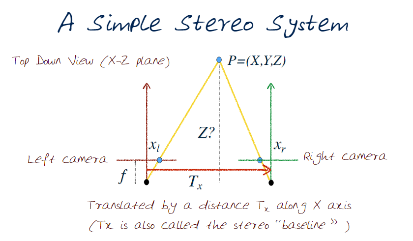
By taking a second image we can now use triangulation to resolve the ambiguity from before.

The idea of stereo vision has been around for a long time.Back in 1838 Sir Charles Wheatstone created a stero viewer where a blocker was placed to seperate each eye's scene. This lead to anaglyphs, where two slighlty different perspectives of the same scene are superimposed on each other in contrasting colors, producing a three-dimensional effect when viewed through two corresponding coloured filters.

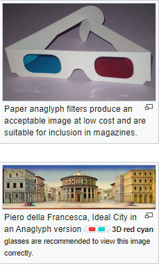
Remember those paper glasses where one lense was red and one was green, those were for viewing anaglyph images. It works by selectively filtering each colour. The red lense selectively passes red colour, and the cyan does the same filtering for the cyan colour. The brain then trys to fuse the two together.

Creating an Analglyph is actually pretty simple. Get two images, a left and right, and convert to greyscale. Then simply create a new canvas and set the blue and green channels to the right image, and the red channel to the left image. That's it

Now let's turn back to our simple stereo image.

Recall our geometric illustrations from before

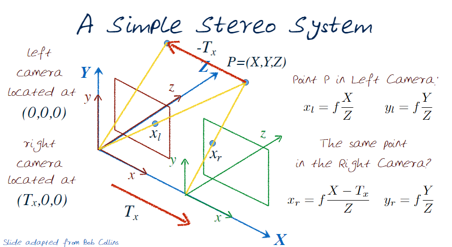
We know that the camera has moved $T_x$ and therefore the point will have moved in the opposite direction (ie $-T_x$) in our geometry. Computing $x_r$ is now straight forward, and $y_r$ hasn't changed. This disparity can be easily formulated as $d = x_l - x_r = f \frac{T_x}{Z}$ we can now express, and solve for, the depth Z as $Z = f \frac{T_x}{d}$

How do we compute disparity? For that we need correspondence, a way to map point from the right image to the same point in the left image. to do this we could use many of the methods we've already covered like feature detection, but this is often above and beyond what is really needed. We introduce the idea of an Epipolar Constraint: rather than search the whole image we reduce our search space to the same line as the point we have as our source. This just says look along the same line in the target image as your source image.

This isn't perfect though. Sometimes you get some black patches with no information. Another problem, which is much more difficult, is occlusion (blockers), this leads to zero matches. The size of the patch also has a large effect.

6 Videos

P6.01 Video Processing

Video is basically a stack of images in Time

Objectives:

1. Relationship between Images and Videos
2. Persistence of vision in playing (and capturing) Videos
3. Extend filtering and processing of images to videos
4. Tracking points in videos

Recall:

• A digital Image has a height (y-axis) and a width (x-axis) which we write as I(x,y)
• Each (x,y) pair has an intensity value
• Resolution is simply h*w

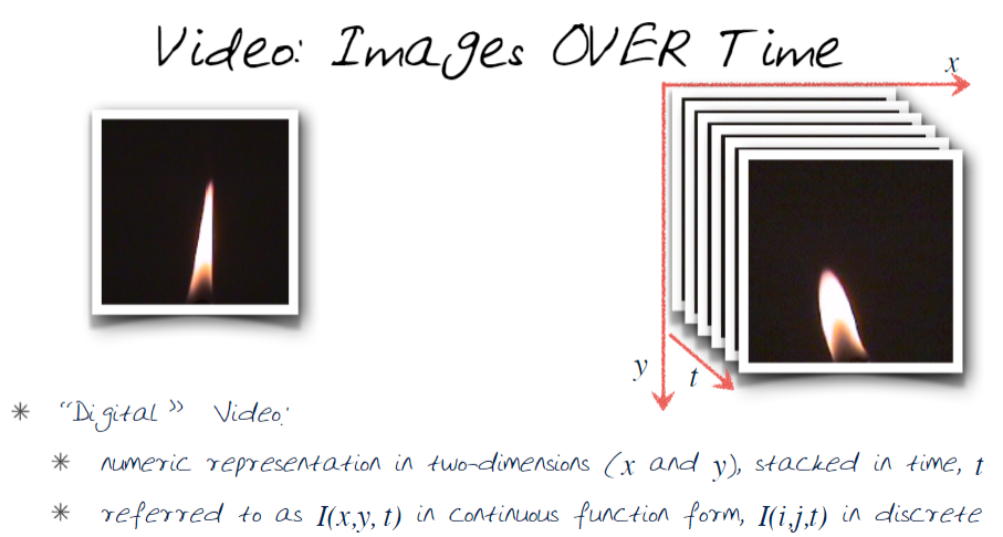
We can extend these now to Video. Let I(x,y,t) = a digital image at a point in time t

When the time delta is less than 1/24, refresh rate, of a second we get the Persistence of vision or illusion of movement. When the refresh rate is higher you may get flickering.

Feature detection is done very much the same as before. Additionally, we can remember their location in the previous frame so as to detect possible changes. This is the direct approach to tracking. The alternative, motion detection, computes the motion at the pixel level between frames (aka optical flow).

P6.02 Video Textures

Goal : How to find similar frames in a video volume to generate longer videos

Objectives

1. Concept of Video Texture
2. Methods used to compute similarity between frames
3. Use of similar frames to find transitions to generate video testures
4. Folding, Cutting, Morphing for Video Testures
5. Some applications of Video Textures

Recall from our previous section that a video is simply a eries of images indexed over time. A video texture is a looping video with a smooth, minimal, unnoticable transition. In order to formulate a video texture we simply look for frames that are highly similar. These frames then form our video endpoints, the frames in between form the bulk of our video.

So how do we define similarity?
Let p & q be the same point in each frame

Method 1 : Euclidian distance metric (L2-Norm)
$d_2(p,q) = \sqrt{ (p_1 - q_1)^2 + (p_2 - q_2)^2 + \dots + (p_n - q_n)^2 }$

Method 2 : Manhattan distance (L1-Norm)
$d_2(p,q) = | (p_1 - q_1) + (p_2 - q_2) + \dots + (p_n - q_n) |$

P6.03 Video Stabilization

Goal : To remove excess shaking/motion in a video

Objectives:

1. Video Stabilization
2. Estimating camera motion
3. Smoothing camera paths
4. Rendering stabilized video
5. Dealing with rolling shutter artifacts

Basic Pipeline:
a. Estimate the camera Motion
b. Stabilize the camera path
c. Crop and re-synthesize

In the old days (1970s) the stedicam was invented. It was a camera mounted on a harness to the photographer. It worked by balancing a counter weight to prevent jagged movements. It mount and allowed the wearer not to need a tripod.

Other methods of optical, or in camera, stabilization include Floating lenses (electromagnets), sensor shifts, Accelerometer with gyroscope and High frequency perturbations using a small buffer. In our discussion we will look at post process stabilization.

We begin by looking for a common area across multiple frames. A crop of the original video. It won't be perfect but it allows us to track the camera motion. one drawback to this is that you may get areas of black if the scene we focus us moves too much. If we focus on a crop that is always within the image bounds then we can avoid the black that occurs from going out of bounds.

Estimating camera motion involves understanding motion models. recall that in panaroramas we want the motion model with the least number of degrees of freedom. The first was translation, second was similarity (translation + scale), third was homography (translation + scale + rotation) with 8 degrees of freedom. It should be noted that homography will produce the best results.

Stabilization

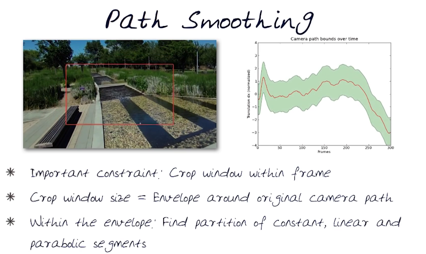
Resynthesize*
Basically this is the recreation of the video using a cropped area along the estimated camera path

P6.04 Panoramic textures

Combining Video textures and panoramas to create panormic video textures

Objectives:

1. Review Video textures
2. Combine textures and panoramas to form panoramic video textures (pvt)
3. Construct panaroma from video
4. Construct video texture from dynamic parts of a scene

What is a PVT?

• A video that has been stiched into a wide field of video
• Appears to play continuously and indefinitely

Recall from panoramas: We take several images and stich them together to form a larger field of view.

How it's done? There are two possible methods.
A) Continuous Approach: Using multiple video frames, register and then align to generate a panorama.
B) Discrete Approach: Take multiple images and place in overlapping areas to generate panorama. Often times both are done on a scene.

Both methods will work.

Video registration: taking each frame we register them and create a wide field of view. This would only create a panorama though. We still need to ensure that the dynamic motion in the scene is captured. For that we use the lessons from video textures. Additionally this texture should be focused on the dynamic areas, not the whole scene.

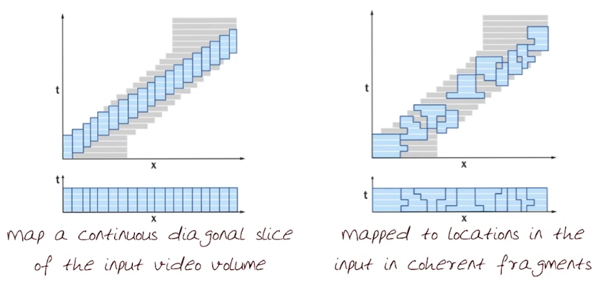
• Map a continuous diagonal slice of the input video volume to the output panorama
• Restricts boundaries to frames
• shears spatial structures across time ( dynamic motion appears linear and moving in one direction )

In order to mitigate the shearing affect we can use cuts, faded and blended, across the diagonal slice of the input frame. these cuts are performed in much the same way as those used in seam carving.

7 Light

P7.01 Light Fields

Goal: To introduce the concepts of a light field and the plenoptic function
How to capture a light field

Objectives:

• Concept of a light field
• Seven parameters of the plenoptic function
• Different types of light fields
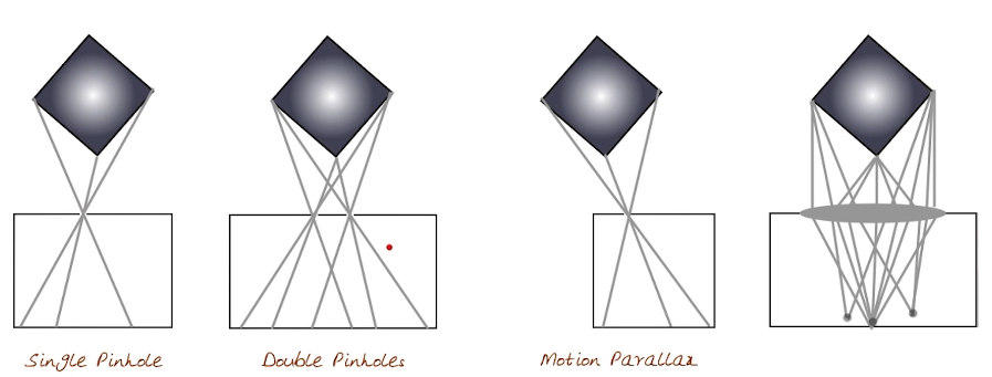
• Scene when viewed from a pinhole and a lens system
• Use of eccentric aperture on a simple lens system
• An array of pinhole cameras
• A 4D light field camera

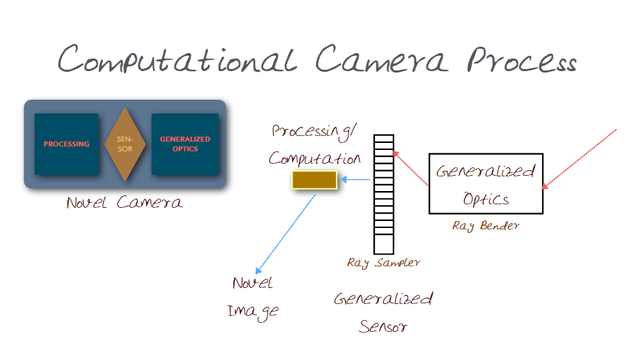
Recall from our earlier conversations that an image captures the light reflecting from an object. Illumination (Light Rays) follow a path from the scene to the sensor. Computation adaptively controls the parameters of the optics, sensor and illumination.

Suppose that we also add the viewing angle co-ordinates ($V_x, V_y, V_z$).
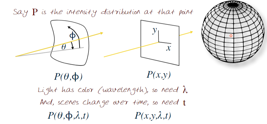
Now we have the plenoptic function
$P_f$ = $P(\theta,\Phi,\lambda,t,V_x,V_y,V_z)$ or $P(x,y,\lambda,t,V_x,V_y,V_z)$

The plenoptic function $P_f$ is measured in an idealized manner by placing an eye at every possible location in the scene $(V_x,V_y,V_z)$ and recording intensity of light rays, wavelength $\lambda$, at time t at every possible angles $(\theta,\Phi)$ around $V_z$ or in terms of (x,y).

Plenoptic (Latin) : Of or relating to all the light, traveling in every direction in a given space. This is the capture/visualization of a 3d holograph which requires 7 diminesions.

If we drop time-t and wavelength-$\lambda$ we can create a hologram like those on a credit cards.

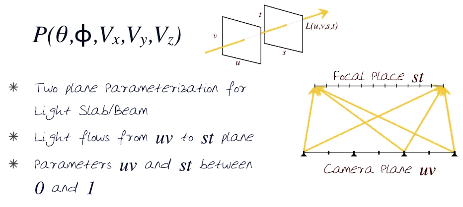
• Rays arriving at one point on the u,v plane are from all points on the s,t plane
• Rays leaving from one point on the s,t plane bound for all points on the u,v plane

In the simplest example we have 2-dimensional light field expressed as $P(\theta,\Phi)$, like a panorama.

Imagine we want to build a pinhole camera using the above idea.

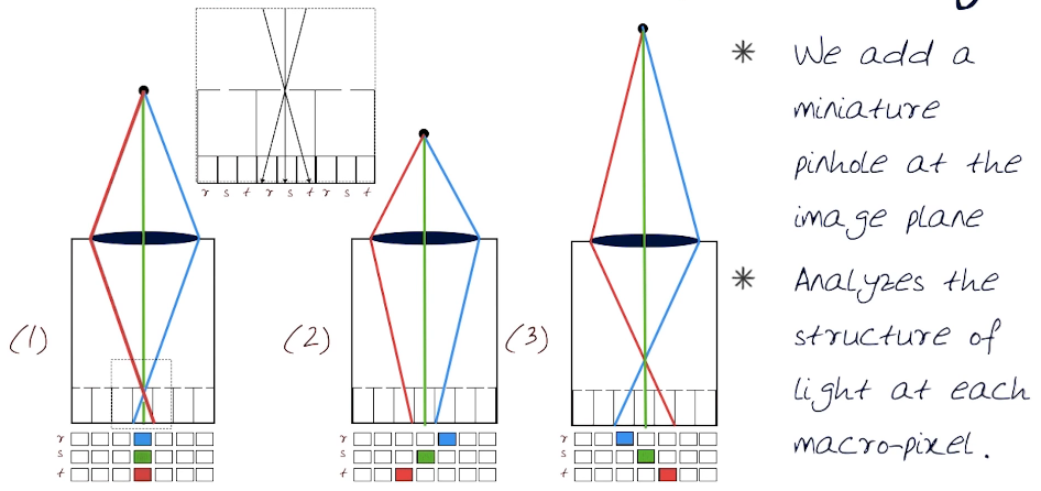
Encoding Direction and intensity using the r-s-t system

P7.02 Projector Camera Systems

Combining a controllable camera and a light source

Objectives:

1. Basics of controlled illumination
2. Use of a projector as a controlled light source
3. Projector-Camera system
4. Projector Callibration
5. Examples of PROCAMS (Projector Cameras)

Recall that a computational photograph begins with a 3d scene (1) and illumination (2).

Lightstage
Imagine an illumination device composed of many lights turning on & off like a strobe light. In addition there is an object in the centre and a camera set to take pictures at multiple points. The key here is to take pics at different points in the light stream. This allows us to produce novel types of images and videos.

3D Scanning using Mobile Phones
A former georgia tech student created an app for iPhone called "Trimensional App" similar in concept to the Lightstage. You go to a dark room and turn on the app. It will shine a light on your face from 4 different angles while taking a photo from each point. Upon completing the app then merges the 4 photo lightsources into a 3 dimensional view of your face.

Given a controlled light we can scan & relight a scene. How can we produce computer controlled light? If we can recall our earlier discussions projectors are controlled light sources that can be manipulated using computers. We simply need to know how to calibrate the projector. We could move the projector after each light burst, but this would be silly when we can simply warp the image.

Obstruction Aware light Can a light source be aware of an obstruction? Yes, but you need multiple light sources.

P7.03 Coded Photography

Cameras that capture additional information about a scene by using controlled patterns built into the imaging process.

Objectives

1. From Epsilon Photography to coded photography
2. Concept/Ideals of coded photography
3. Coded Aperture
4. Flutter shutter camera

Recall from our earlier discussion on Epsilon Photography: Multiple sequential photos are taken while changing some parameters by a small, epsilon, amount. Then they are fused together to produce a richer representation. HDR images are one example of this, Panoramas were another.

• Control Exposure: Control light in Time
• Coded Aperture: Control light near the sensor
• Coded Illumination: Control light in the scene
• Coded sensing: Coded intensities

Coded Photography and Epsilon have similarities:

• Coded photography encodes the photographic signal and post-capture decoding for improved scene analysis.
• Encoded photography: successive frames may have slight variations
• Coded Photography: Neighboring pixels may have different variations.
  • Controlling light over time and/or space
  • preserve details about the scene in the recorded image

Suppose we want to determine the depth of objects in an image. Recall that the distance of an object from the lens has an impact on the focal point. If the lens position is held constant and the object moves further away the focal point nears the lens and becomes blurred in the final image. The further the object is the more blurry it becomes. Now given an image we can determine the depth of the objects by looking at the level of blur in different areas of an image.

This presents some challenges. How to discriminate between defocus blurring? How do we undo a defocus type of blur?
Possible Approaches:

Defocusing as a local convolution: Requires calibrations of blur kernels at different depths(k).
Let k=1,2,3.. be the depth

• Choose a local subwindow $y_k$
• Calibrate blur kernels at depth $f_k$
• Sharpen the subwindow $x$ using a convolution

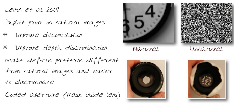
We could use a coded aperture (implemented as a mask)

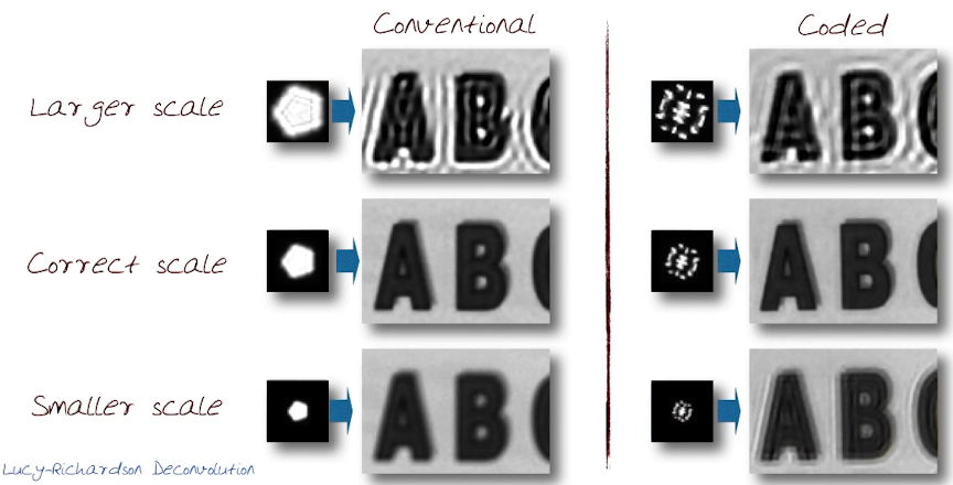
Can these masks be created analytically? In order to answer this question we need to understand the discrimination of the mask. As it turns out the greater allowance radiating from the centre of the mask can be measured as the discrimination

Coded Aperture:
Pros

• Image and depth in single shot
• No loss of resolution
• Simple modification to lens
• deconvolution increases depth of field

Cons

• Depth is coarse
• loss of light

8 - Additional Required Readings

P8.01 Interactive Digital Photomontage

Main:
Interactive digital photomontage
Paper website
Paper Video

Secondary:
All Smiles

Summary:
Consider a photo of a group of people. Often times some the camera captures some people very well and others not so well. Could we fuse the best person from each image into a single composite image?

Pipeline: Select a starting image for your composite.
For each other image

• select a region that is better than the composite
• perform a graph cut on the region
• integrate the graph cut region into the composite

P8.02 Accidental Pinhole and Pinspeck Cameras

Main:
Interactive digital photomontage
Paper website

Embedded Video Below

%%HTML
<div align="middle">
    <video width="80%" controls>
          <source src="CS6475_resources/CVPR2012.mp4" type="video/mp4">
    </video>
</div>

P8.03 Eulerian Video Magnification

Main:
Eulearian Video Magnification
Paper website
Video

Secondary:
Motion Magnification

Summary: First we take a standard video sequence as input then decompose it into different spatial frequency bands using a Laplacian pyramid

from IPython.display import YouTubeVideo
# a talk about IPython at Sage Days at U. Washington, Seattle.
# Video credit: William Stein.
YouTubeVideo('ONZcjs1Pjmk')

P8.04 Poisson Image Editing and Drag-and-Drop Pasting

Main:
Patch Match
Paper website

Secondary:
Drag and Drop

Summary: First we take a standard video sequence as input then decompose it into different spatial frequency bands using a Laplacian pyramid

P8.05 PatchMatch and Content Aware Fill

Main:
Patch Match
Paper website

Summary: First we take a standard video sequence as input then decompose it into different spatial frequency bands using a Laplacian pyramid

%%HTML
<div align="middle">
    <video width="80%" controls>
          <source src="CS6475_resources/PatchMatchAndContentAwareFill.mp4" type="video/mp4">
    </video>
</div>