CS7280 Network Science¶

Class Details¶

Teacher: Constantine Dovrolis

Course Website:

https://faculty.cc.gatech.edu/~dovrolis/Courses/NetSci/

Extra Material:

http://networksciencebook.com/
https://www.cs.cornell.edu/home/kleinber/networks-book/networks-book.pdf
York University Webpage
- https://www.eecs.yorku.ca/~papaggel/courses/eecs4414/
- https://www.eecs.yorku.ca/~papaggel/courses/eecs4414/docs/lectures/03-network-models.pdf
- nice overview/summary of various models discussed in this class
University Of Nebraska
- Statistical Analysis of Networks
- https://bigdata.unl.edu/documents/ASA_Workshop_Materials/Tutorial%20Statistical%20Analysis%20of%20Network%20Data.pdf
Jackson State University
- Theoretical Models G(n,p) ER Models, scale-free Networks, small worlds(Watts-Strogatz)
- https://www.jsums.edu/nmeghanathan/files/2016/01/CSC641-Sp2016-Module-5-TheoreticalNetworkModels.pdf

Student objectives/takeaways:

What “network science” means,
- how it relates to other disciplines (graph theory, data mining, machine learning, etc),
- how it is useful in practice
How to detect, quantify and interpret important properties of real networks,
- such as power-law degree distribution,
- “small world” efficiency and clustering,
- assortativity, hierarchy, modularity, and others
Learn how to identify the most important nodes and links in a network through network centrality metrics and core identification algorithms
Design and analyze algorithms that compute “communities” of highly clustered nodes,
- learn how to compare such algorithms
Appreciate the value of network modeling, and learn several approaches to model a static or dynamic network
Understand the “network inference” problem and learn statistical and machine learning methods that estimate a network from noisy data
Understand how representation learning (and deep learning in particular) is applied to network science
Learn how to model and predict network epidemics, influence, cascades, and other “spreading” phenomena
Understand how the structure (topology) of a network affects the function and dynamic activity on that network
Become familiar with several state-of-the-art research directions in network science

Grading :
This course will use the following grade breakdown:

Projects (5 in total): 65%
One quiz for each lesson (14 in total): 35%
Note Knowledge Check (KC) are NOT graded

The final grade will be determined based on your final weighted grade average (no "curving"), as follows:

A: 100-85%
B: 85-70%
C: 70-60%
D: 60-50%
F: Below 50%

Course consists of 5 Modules -- and a total of 14 Lessons:

L0 Introduction¶

What is Network Science¶

Chapter 1: http://networksciencebook.com/chapter/1#networks

Understanding connectivity. In a nutshell this is what Network science is really all about. It could be tangible like the connectivity of wires carrying electricity, it could be intangible, like the global economy.

Understanding Connectivity also requires understanding their complexity, and vulnerability. How local failures in one country travel and reverberate to it's economic partners and their partners and beyond.

Some examples of networks:

network encoding the interactions between genes, proteins, and metabolites
wiring diagram capturing the connections between neurons, called the neural network
The sum of all professional, friendship, and family ties, often called the social network,
Communication networks, describing which communication devices interact with each other,
The power grid, a network of generators and transmission lines
Trade networks maintain our ability to exchange goods and services

Modern Network science traces itself back to two papers published in 1959, by Paul Erdos and Alfred Renyi. Although it had very humble beginnings, it rose rapidly with the world wide web and advances in technology that could handle larger and larger maps of networks.

Characteristics of Network Science:

Interdisciplinary Nature: The language of Networks allows for commonality across areas. Centrality was first constructed to describe growing social networks but today it is used to identify high traffic nodes on the internet.
Empirical and Data Driven: Tools are developed and tested on real phenomena
Computational Nature

Complex Systems have:

Many and heterogeneous components
Components that interact with each other through a (non-trivial) network
Non-linear interactions between components

Network science maps highly complex systems into a graph -- an abstraction that we can analyze mathematically and computationally to ask a number of important questions about the organization of this neural system.

Some example architectures

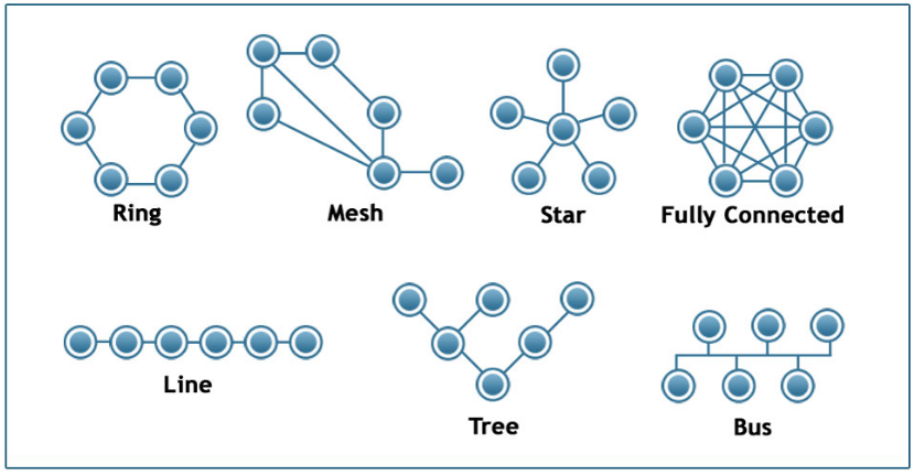
Ring architecture provides two disjoint paths between every pair of nodes.
Line, Tree, and Star architectures require the fewest number of links but they are highly vulnerable when certain nodes or edges fail.
The Fully Connected architecture requires the highest number of links but it also provides the most direct (and typically faster) and resilient communication.
The Mesh architecture provides a trade-off between all previous properties.

We will study such influence or “information contagion” phenomena

important but still open research question is whether it is possible to develop algorithms that can identify influential spreaders of false information in real-time

We will also study problems at the intersection of Network Science and Machine Learning.

Machine Learning models have been used to predict previously unknown interactions between drugs and genes.

Roots of Network Science

Key topics that each of these disciplines contributed to Network Science.

Graph theory: Study of abstract (mostly static) graphs
Statistical mechanics: Percolation, phase transitions
Nonlinear dynamics: Contagion models, threshold phenomena, synchronization
Graph algorithms: Network paths, clustering, centrality metrics
Statistics: Network sampling, network inference
Machine learning: Graph embeddings, node/edge classification, generative models
Theory of complex systems: Scaling, emergence

There are two main differences however

First, Network Science focuses on real-world networks and their properties
Second, Network Science provides a general framework to study complex networks independent of the specific application domain

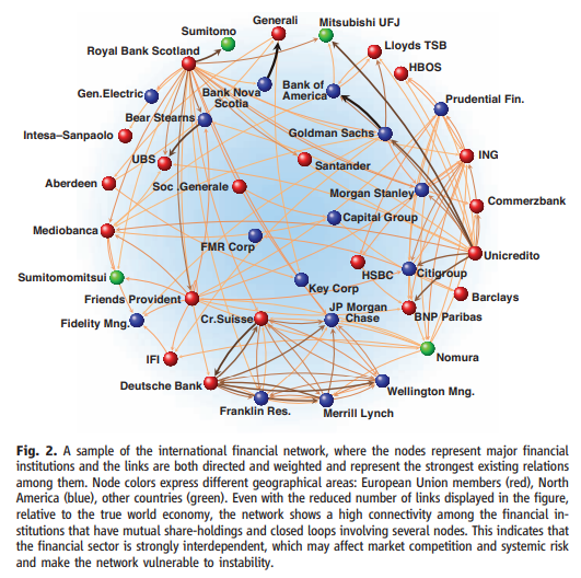
Economic Networks: The new Challenges¶

Paper: https://www.sg.ethz.ch/publications/2009/schweitzer2009economic-networks-the/

Extracting network topology from reported data, in particular for aggregated economic data, is very difficult. This is particularly true for the banking sector, where detailed accounts of debt-credit relations are not publicly available
Although a topical subject, most theoretical and empirical methods are not suited to predicting cascading network effects

L1A: Graph Theory - Review¶

Chapter-2 from A-L. Barabási, Network Science
Chapter-2 from D. Easley and J. Kleinberg, Networks, Crowds and Markets

Birth of graph theory was in 1736 when Leonhard Euler worked on the bridge of Königsberg problem. Incidentally, Konengsburg is now Kalinangrad in modern day Russia. In this problem each bridge represents an edge and the endpoints, landmass, is a node. His goal was to cross each bridge just once. A solution to such types of problems is now called a Eulerian path.

Terminology

A graph, or network, represents a collection of dyadic relations between a set of nodes
- these nodes are denoted as V, for the set
- the relations are referred to as edges or links and denoted by E
- So an edge (u,v) is an element of E and represents a relation between nodes u & v in V
Graphs are denoted G=(V,E)
- Typically we do not allow edges between a node and itself.
- Simple graphs are undirected and unweighted
- max number of edges are n(n-1)/2 or $n \choose 2$ n choose 2
Density of a graph is the ratio of edges m to the max number of edges
The degree of a node v is the number of connections to v, ie the number of edges that connect to it

Representation¶

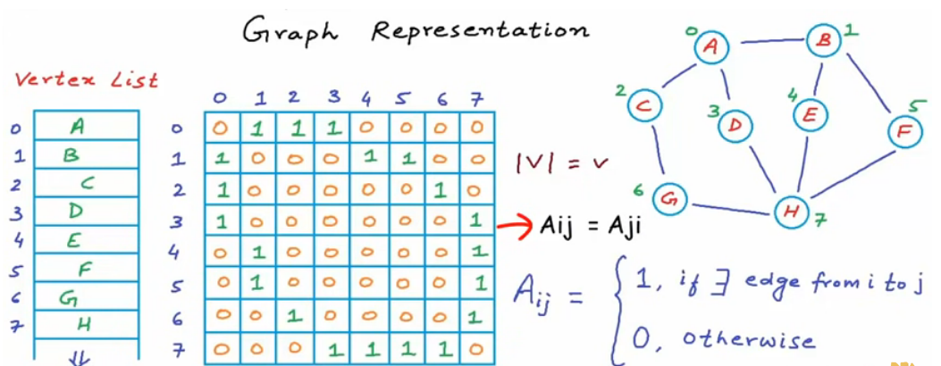
A graph is often represented either with an Adjacency Matrix
- this representation requires a single memory access to check if an edge exists
- but it requires $n^2$ space (because every edge is included twice)
- this representation also allows us to use tools from linear algebra to study graph
Sparse Graph:
- A graph is sparse if the number of edges m is much closer to the number of nodes n than to the maximum number of edges
- meaning the adjacency matrix of a sparse graph is mostly zeros

Walks, Paths, Cycles

A Path is a series of ordered edges that visits nodes only once, all nodes are distinct
A Walk is a path that visits at least 1 edge more than once
A cycle is a path that starts and ends at the same node

An undirected graph is connected if there is a path from any node to any other node
A directed graph is weakly connected IFF the graph is connected when the direction of edges between nodes is ignored

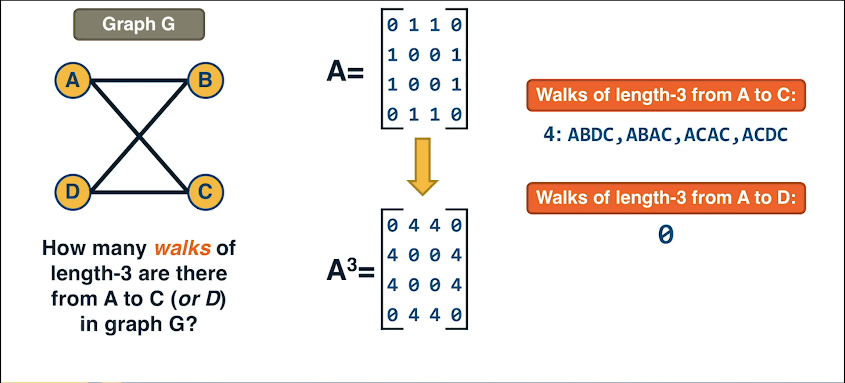
Consider: How can we efficiently count the number of walks of length k between nodes s and t?

Turns out this is just $A^k$ where A is the adjacency matrix.
Let's consider why.
For k = 1 the number of walks is either 0 or 1 depending on whether or not s,t are directly connected
For k > 1 it gets a bit tricker. For k-1 the number of walks is the number of walks of length k-1 that end at a node that connects to t. Thus the number of walks of length k that end at v is given by the element (s,t) of $A^k$

$\sum_{v \in V} A^{k-1}(s,v) A(v,t) = A^k(s,t)$

In this course, we will focus instead on complex graphs that do not fit in any of these special classes. However, we will sometimes contrast and compare the properties of complex networks with some regular graphs.

Simple Graph Properties

Tree: m=n-1, connected, no cycles
k-regular graph: a network in which every vertex has the same degree k
Complete graph: aka Clique is a special case of a regular network in which
- every vertex is connected to every other vertex

Directed Graphs

corresponding adjacency matrix may no longer be symmetric
common convention is that the element (i,j) of the adjacency matrix is equal to 1 if the edge is from node i to node j
node degree:
- in-degree of v: the number of incoming connections to a node v
- out-degree of v: the number of outgoing connections from v

In some cases the edge weights represent capacity (especially when there is a flow of some sort through the network). In other cases edge weights represent distance or cost (especially when we are interested in optimizing communication efficiency across the network).

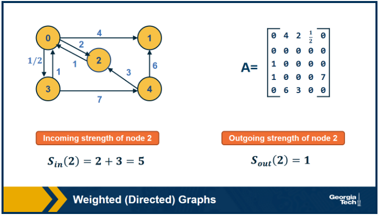
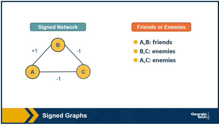
In signed graphs, the edge weights can be negative, representing competitive interactions. For example, think of a network of people in which there are both friends and enemies (as shown in the visualization above).

Connected Components¶

A connected component or simply component of an undirected graph is a subgraph in which each pair of nodes is connected with each other via a path. A graph need not be connected.

Breadth-first-search (BFS) traversal from node s can be used to find the set of nodes in the connected component that includes s. Starting from any other node in that component would result in the same connected component.

If we want to compute the set of all connected components of a graph, we can repeat this BFS process starting each time from a node s that does not belong to any previously discovered connected component. The running-time complexity of this algorithm is 𝝝(m+n) time because this is also the running-time of BFS if we represent the graph with an adjacency list.

Strongly Connected Components¶

In directed graphs, the notion of connectedness is different: a node s may be able to reach a node t through a (directed) path – but node t may not be able to reach node s.

A directed graph is strongly connected if there is a path between all pairs of vertices. A strongly connected component (SCC) of a directed graph is a maximal strongly connected subgraph.

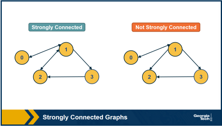
If the graph has only one SCC, we say that it is strongly connected. How would you check (in linear time) if a directed graph is strongly connected?

Consider running BFS on both G and G' where G' has the reverse edges of G. if all nodes are reached in both cases then it is stronly connected.

Directed Acyclic Graphs - DAG¶

A directed acyclic graph is a directed graph with no cycles.

1) A directed graph is a DAG IFF it can be topologically ordered
- ie the vertices can be arranged as a linear ordering
2) A DAG must include at least one source node, a node with zero incoming edges
3) if a graph is a DAG then it must have a topological ordering

Dijkstra's Shortest Path Algo¶

In many graph problems we are usually interested in the shortest path between two nodes, because this represents the most efficient way to move in a network.

In an unweighted network all paths are considered to have the same weight, 1. Thus the shortest path is just the number of edges. When a network is weighted, the weight of each edge is it's length or cost, for this we use dijkstra's algorithm. The only caveat here is that the weights must be positive.


d_s = 0
d_i = inf  for i != s
T = V
for i=0 -> n-1 
    choose v_m in T with min(d_m)
    for each edge (v_m,v_t) with v_t in T
        if d_t > d_m + C_m,t
            then d_t = d_m + C_m,t
    T = T-v_m

The key idea in the algorithm is that in each iteration we select the node m with the minimum known distance from s – that distance cannot get any shorter in subsequent iterations. We then update the minimum known distance to every neighbor of m that we have not explored yet, if the latter is larger than the distance from s to m plus the cost of the edge from m to t.

If you have negative weights then you need to use the Bellman-Ford algorithm, which is a classic example of dynamic programming. The running-time of Bellman-Ford is O(mn), where m is the number of edges and n is the number of nodes. On the other hand, the running time of Dijkstra’s algorithm is O(m + n log_n) if the latter is implemented with a Fibonacci heap (to identify the node with the minimum distance from s in each iteration of the loop).

L1B: Concepts Review¶

Random Walks¶

These are handy when we know we are only dealing with a partial map. Our line of sight is limited to our current node and it's edges and neighbours. A web page is an example of this as it may be filled with links that serve as an edge to a neighbouring node. Of course we won't know what links are contained in the neighbouring node until we visit it. In such a situation it is useful to perform a random walk.

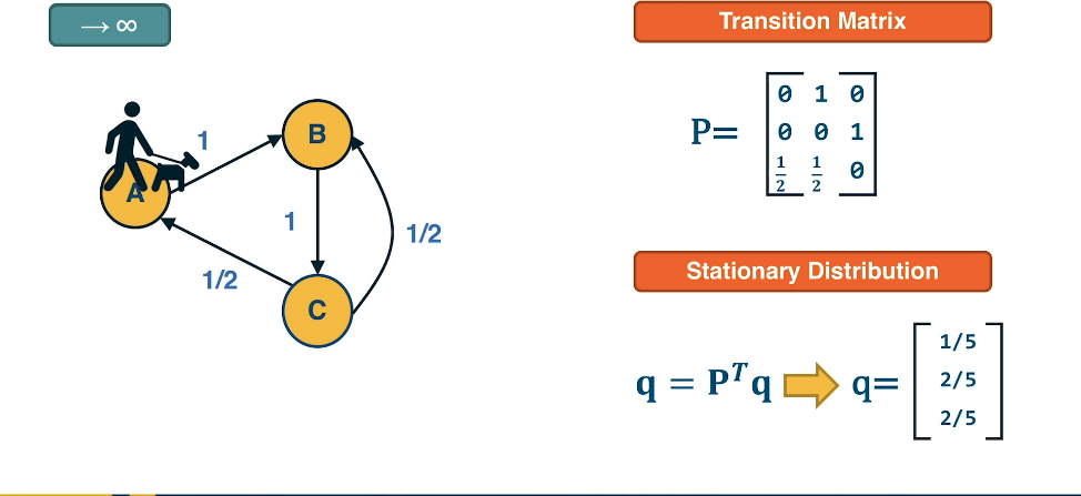
Consider an algo called walker that is stationed at node v. The walker picks a random neighbour of v and moves there. In an unweighted graph the probability of choosing an fixed but arbitrary edge is 1/k where we assume k outgoing edges. If however, the network is weighted then the probability becomes a function of the weight. We will denote this transition probabilities by the matrix P. Where the (i,j) element is the probability that the walker moves from node i to node j.

For the unintiated this situation is what's called a Markov Process.

Suppose our walker is sent on a random walk. It'll move from node to node to node. every so often it will land on a node it's previous visited. It will also keep count of the number of time it visits a node. In doing so something will emerge ... we will see a distribution appear ... or what is commonly called a stationary distribution.

Can we calculate this distribution using our transition matrix?

Let $q_t$=vector of probabilities for each node at time t
Let $P$=Transition matrix
Then, for each step in the random walk
- $q_{t+1}=P^T q_t$
- ie Pr(curr_node=i) = $\sum_j$ Pr(edge(j,i)) x Pr(prev_node=j)
- Probability of landing on i is the probability of currently at a neighbour of i, denoted by j, times the transition probability
As t increases the probability values of $q_t$ will converge asymptotically.
Note that sum of elements in $q_t$ must always sum to 1 at all times

Theorem: Let q be the stationary distribution expressed as a column vector. It satisfies the relationship $P^T q = q$ for transition matrix P.

This is true because, irrespective of the starting state, eventually equilibrium must be achieved. The transient, or sorting-out phase takes a different number of iterations for different transition matrices, but eventually the state vector features components that are precisely what the transition matrix calls for. So, subsequent applications of "P" do not change the matured state vector.

Recall from linear algebra that a transition matrix T has an eigenvector v if $Tv = \lambda v$ for eigenvalue $\lambda$. From this we can see that the eigenvectors of $P^T$ are the stationary distribution expressed as column vectors where $\lambda=1$. An important result of this is that, in undirected and connected networks, a stationary distribution always exists. It is not, however, necessarily unique.

Max Flow-Min Cut¶

Define A flow network is a weighted and directed graph. The weighting here can be interpreted as the capacity of an edge. An example of this is a water pipe. A pipe has a max capacity, but of course it doesn't always have to be maximized in order to be used.

Min-Cut
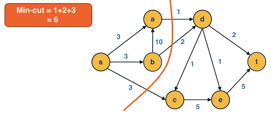
Problem: Given a flow network, a weighted directed graph, with a source node s and a sink node t, we define a cut(s,t) of the graph as the set of edges which, when removed, will disrupt all possibles paths from s to t.

The min cut is simply the cut with the least possible weight that disrupts all possible paths from s to t

Max-Flow

The max-flow problem refers to computing the maximum amount of flow that can originate at s and terminate at t, subject to the capacity constraints and the flow conservation constraints.

Flow-Conservation = the flow into a node is equal to the flow out of a node. This also holds true for the entire network as well sink all flow originates at the source s and ends at t.
Capacity Constraint = flow <= capacity , you cannot exceed the capacity

Ford-Fulkerson algorithm takes O(mC) where m=number of edges and C is the max capacity.

This algorithm works by constructing a residual network, which shows at any point during the execution of the algorithm the residual capacity of each edge. In each iteration, the algorithm finds a path from s to t with some residual capacity (we can use BFS or DFS on the residual network to do that). Suppose that the minimum residual capacity among the edges of the chosen path is f. We add f on the flow of every edge (u,v) along that path, and decrease the capacity of those edges by f in the residual network. We also add f on the capacity of every reverse edge (v,u) of the residual network. The capacity of those reverse edges is necessary so that we can later reduce the flow along the edge (u,v), if needed, by routing some flow on the edge (v,u).

Theorems

A: mincut(s,t) $\ge$ maxflow(s,t)
- for any cut(L,R) $s \in L$ and $t \in R$ has capacity >= any flow from s to t
B: If f*=maxflow(s,t) the network can be partitioned in two sets of nodes L and R with $s \in L$ and $t \in R$ such that
- all edges from L to T have flow = capacity
- all edges from R to L have flow = 0

So edges from L to R define a cut(s,t) with capacity = maxflow(s,t) and because of Part A this cut is mincut(s,t).

This mincut(s,t) = maxflow(s,t)

Bipartite Graphs¶

Another important class of networks is bipartite graphs. Their defining property is that the set of nodes V can be partitioned into two subsets, L and R, so that every edge connects a node from L and a node from R. There are no edges between L nodes – or between R nodes.

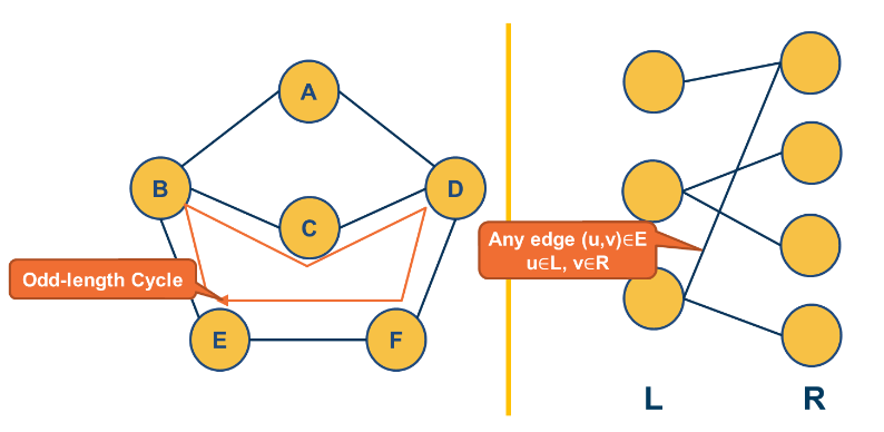
Suppose you want to create a “recommendation system” for an e-commerce site. You are given a dataset that includes the items that each user has purchased in the past. You can represent this dataset with a bipartite graph that has users on one side and items on the other side. Each edge (user, item) represents that that user has purchased the corresponding item.

How would you find users that have similar item preferences?

This question can be answered by computing the “one-mode projection” of the bipartite graph onto the set of users. This projection is a graph that includes only the set of users – and an edge between two users if they have purchased at least one common item. The weight of the edge is the number of items they have both purchased.

How would you find items that are often purchased together by the same user? Knowing about such “similar items” is also useful because we can place them close to each other or suggest that the user considers them both.

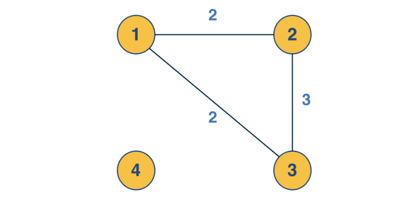
This can be computed by the “one-mode projection” of the bipartite graph onto the set of items. As in the previous projection, two items are connected with a weighted edge that represents the number of users that have purchased both items.

Co-citation and Bibliographic Coupling¶

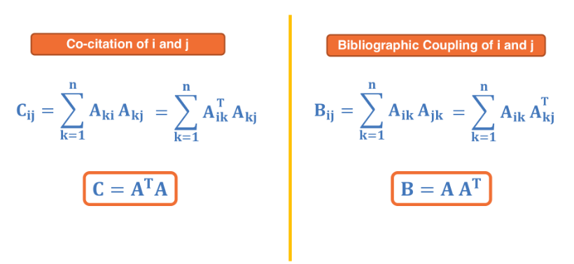
One-mode projections can also be computed using the adjacency matrix A that represents the bipartite graph.

Suppose that the element (i,k) of A is 1 if there is an edge from i to k – and 0 otherwise.

The co-citation metric $C_{ij}$ for two nodes i and j is the number of nodes that have outgoing edges to both i and j. If i and j are items, then the co-citation metric is the number of users that have purchased both i and j.

On the other hand, the bibliographic coupling metric $B_{ij}$ for two nodes i and j is the number of nodes that receive incoming edges from both i and j. If i and j are users, then the bibliographic coupling metric is the number of items that have been purchased by both i and j.

Graph Terminology¶

Terminology

{network,node,link} are used when describing real world networks like an electrical grid or WWW-world wide web
{graph,vertex,edge} are used when describing a mathematical representation

Degree - refers to the number of links a node has to other nodes
- the total number of links in a network is the total sum of each nodes degrees

L3 - Degree Distribution and The “Friendship Paradox”¶

Degree Distribution - ER Graphs¶

Define
The degree distribution of a given network shows the fraction of nodes with degree k, (here k is like the x-axis). Alternatively you can also think of it as the probability distribution of degrees for all nodes.

Recall the idea of Statistical Moments

first moment is also known as the mean
- $\bar{k} = \sum k \cdot p_k$
second moment is
- $\bar{k^2} = \sum k^2 \cdot p_k$
Variance is second moment minus first squared
- $\sigma_k^2 = \bar{k^2} - (\bar{k})^2 $

Analysis of larger networks can become tedious when looking at a density function so we will often use the Complementary Cumulative Function C-CDF. Note this is not the same as the CDF that is normally used in most stats classes. It's the opposite.

C-CDF is defined as

$\bar{P_k} = Pr(degree \ge k) = \sum p_x \text{ where } x \ge k $

Here are Two Special Degree Distributions that we will examine in several cases

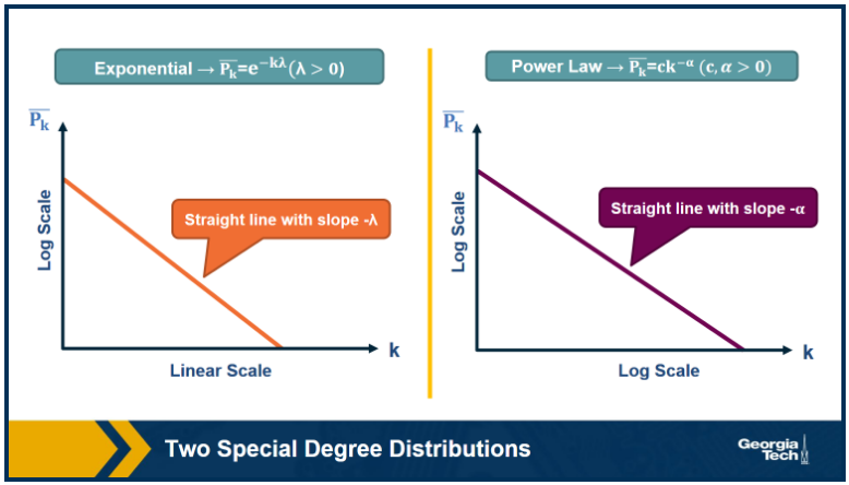
Note that C-CDF plots are often shown using a logarithmic scale at the x-axis and/or y-axis. When the C-CDF decays exponentially fast, then the log-linear plot (left) appears as a straight line with slope $-\lambda$. The avg deg is such a network will be $1/\lambda$.

In other networks the C-CDF decays with a power law of k. For say $\alpha=2$, the probability to see a node with degree at least k drops proportionally to $1/k^2$. In a log-log plot (right) this distribution will appear as a straight line with slope $\alpha$. These types of networks are called scale free and we will examine them later.

Let's look at a small example. Here is bipartite network of sex buyers and sellers, escorts. In the top row we see the probability density functions of the node degrees. The plots in the bottom row are the C-CDF in log-log scale.

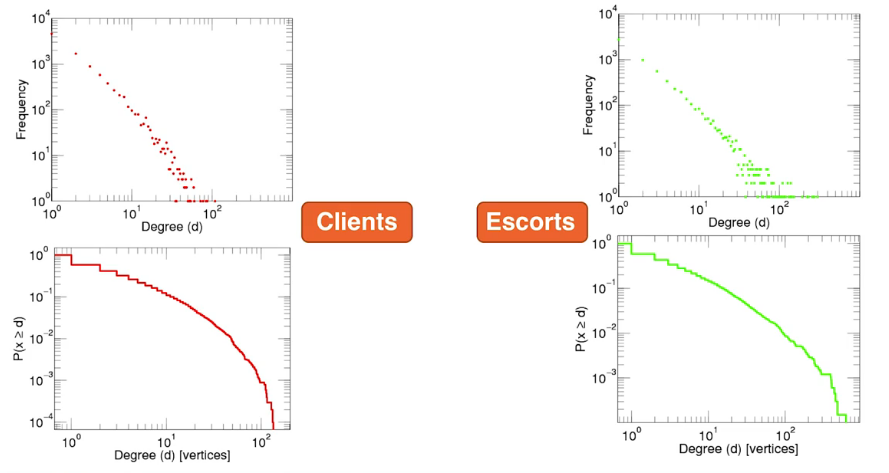
From: https://journals.plos.org/ploscompbiol/article?id=10.1371/journal.pcbi.1001109#pcbi.1001109.s001

Focus for a moment on the chart at the bottom right, which is the C-CDF of the escorts. Although it isn't actually a straight line it is approximately straight up to the point $10^{-3}$. Interestingly is drops off at about this point. Looking back up at the degree density we can see that there are a few outlier escorts with a higher number of degrees. It is these escorts or network hubs that contribute signficantly towards epidemic spreads.

Friendship Paradox¶

In an informal tense, The friendship paradox is the idea that "On avg your friends have more friends than you"

In a formal tense: The average degree of a node's neighbour is higher than the average node degree.

Let's now take a look at how to derive this

Suppose we randomly select an edge from a network. Furthermore suppose we randomly pick one of it's end points (stubs). Then what is the probability that the selected node is of degree k?

If the degrees of connected nodes are indepently distributed then this is rather straight forward

$q_k$ = ( num nodes with degree k ) x ( probability an edge connects to a specific node of degree k)
$= np_k \frac{k}{2m}$
$= \frac{kp_k}{2m/n}$
$= \frac{kp_k}{\bar{k}}$
This says that the probability that a randomly chosen stub connects to a node of degree k is proportional to both k and the probability that a node has degree k.

This means that, for nodes with degree k > $\bar{k}$, it is more likely to sample one of their stubs than the nodes themselves. The opposite is true for nodes with degree k < $\bar{k}$.

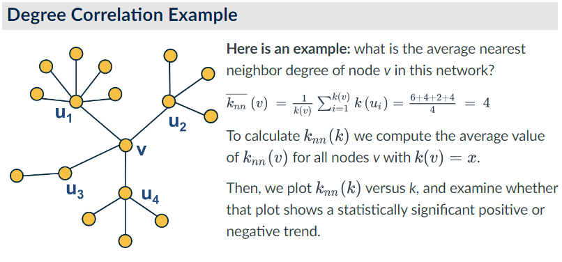
Based on the previous derivation, we can now ask: what is the expected value of a neighbor’s degree? Note that we are not asking for the average degree of a node. Instead, we are interested in the average degree of a node's neighbor. This is the same as the expected value of the degree of the node we select if we sample a random edge stub. Lets denote this expected value as $k_{nn}$.

The derivation is as follows.

$\large \overline{k_{nn}} = \sum_{k=0}^{max(degree)} k q_k = \sum_k k \frac{kp_k}{\bar{k}} = \frac{\sum k^2 p_k}{\bar{k}} = \frac{\bar{k^2}}{\bar{k}} = \frac{(\bar{k})^2 + (\sigma_k)^2}{\bar{k}} = \bar{k} + \frac{\sigma_k^2}{\bar{k}}$

We can now give a mathematical statement of the friendship paradox: as long as the variance of the degree distribution is not zero, and given our assumption that neighboring nodes have independent degrees, the average neighbor’s degree is higher than the average node degree.

The difference between the two expected values (i.e., $\frac{\sigma_k^2}{\bar{k}}$ ) increases with the variability of the degree distribution.

Consider the following two networks in the case of the friendship paradox.

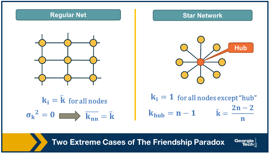
In the left graph all nodes have the same degree, thus the degree variance would be 0. In the right graph we see an infintely large star network with one hub node and many nodes connecting to it. In the left graph the degree variance is 0 and thus every neighbour has the same number of degrees. In the right graph the degree variance grows as n increases. This would also imply that the difference between the avg node degree and the avg neighbour degree is also diverging.

G(n,p) model & ER Graphs¶

Let's consider now the simplest random graph model and its degree distribution.

This model is referred to as G(n, p) and it can be described as follows:

the network has n nodes
and p is the probability that any two distinct nodes are connected with an undirected edge

The model is also referred to as the Gilbert model, or sometimes the Erdős–Rényi (ER) model, from the last names of the mathematicians that first studied its properties in the late 1950s.

Note that the G(n,p) model does not necessarily create a connected network – we will return to this point a bit later.

Note that the number of edges m in the G(n,p) is a random variable. The expected number of edges is $p \frac{n(n-1)}{2}$ , the average node degree is $p(n-1)$, the density of the network is p and the degree variance is $p(1-p)(n-1)$. These formulas assume that we do not allow self-edges.

The degree distribution of the G(n,p) model follows the Binomial(n-1,p) distribution because each node can be connected to n-1 other nodes with probability p.

In the G(n,p) model there are no correlations between the degrees of neighboring nodes. So, if we return to the friendship paradox, the average neighbor degree at a G(n,p) network is $\overline{k_{nn}} = \overline{k}+(1-p)$ (using the Binomial distribution) -- or $\overline{k_{nn}} = \overline{k} + 1$ (using the Poisson approximation when p < 1).

In other words, if we reach a node v by following an edge from another node, the expected value of v’s degree is one more than the average node degree.

One may recall from statistics class many years ago that the binomial distribution can be approximated by the Poisson distribution as long as p is much smaller than 1. In network terms this means that the approximation should hold for a sparse graph where the avg degree p(n-1) is much lower than n, the size of the network.

Recall, the Poisson distribution is given by

$\large p_k = e^{-\bar{k}} \frac{k^{-k}}{k!}$ for k = 0,1,2,...
$\large \bar{k} = p(n-1) $
$\large \sigma_k^2 = \bar{k} $

You may also recall that $1/k!$ decreases very rapidly making the distro converge quickly as well. Why use poisson? Just convenience really. Its easier to work with one parameter $\bar{k}$, the avg node degree.

There is no guarantee that the G(n,p) model will give us a connected network though, even when p > 1. if p is close to zero the network will contain many small components. Which often begs the question: how large is the largest connected component LCC of the G(n,p) model?

https://www.youtube.com/watch?v=mpe44sTSoF8

Suppose we fix n at n=1000. when the avg node degree $\overline{k}$ is small so is p since $p \approx \bar{k}/n $, then the connected components will also be small, say 2-3 nodes at best. In fact most nodes may be isolated in their own connected component. As we let the avg node degree increase then the connected components will grow larger as well. so long as $\bar{k}/n$ is less than 1 we may not see any cycles.

When $\bar{k}/n$ crosses the threshold of 1, meaning the probability that any two distinct nodes are connected is greater than 1, the connected components are quite large and may very well include cycles. If you watch the video you'll notice that after the 1 threshold is crossed the largest component is growing larger and larger. Any further connections added are almost certainly added to it in some way. Eventually at some point there will be a single fully connected component.

Suppose that S is the probability that a node belongs in the LCC. ie S is the expected value of the fraction of network nodes that belong in the LCC. Then $\bar{S} = 1-S$ is the probability that a node does NOT belong in the LCC.

This can also be written $\bar{S} = ((1-p) +p \cdot \bar{S})^{n-1}$

The first term refers to the case that a node v is not connected to another node, while the second term refers to the case that v is connected to another node that is not in the LCC.

Since, $p = \frac{\bar{k}}{n-1}$ the last equation can also be written as follows

$\large \bar{S} = (1 - \frac{\bar{k}}{n-1} ( 1 - \bar{S}))^{n-1} $
taking the natural log of each side yields
$\large ln \bar{S} = (n-1) ln(1 - \frac{\bar{k}}{n-1} ( 1 - \bar{S}))$
which we can reduce to
$\large \approx - (n-1) \frac{\bar{k}}{n-1} ( 1 - \bar{S})$
$\large 1-e^{-\bar{k}S}$

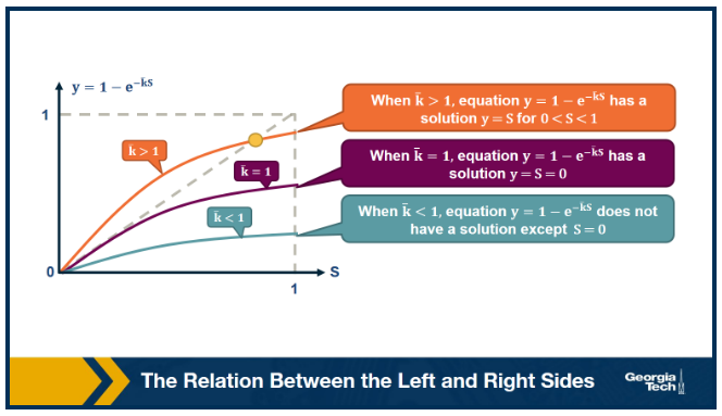
The visualization shows the relation between the left and right sides of the previous equation, i.e., the relation between S and $1-e^{-\bar{k}S}$.

The equality is true when the function $y = 1-e^{-\bar{k}S}$ crosses the diagonal x=y line.

Note that the derivative of y with respect to S is approximately when S approaches 0.

So, if the average degree is larger than one, the function y(S) starts above the diagonal. It has to cross the diagonal at a positive value of S because its second derivative of y(S) is negative. That crossing point is the solution of the equation $y = 1-e^{-\bar{k}S}$. This means that if the average degree is larger than one ($\bar{k} > 1$), the size of the LCC is S > 0.

One the other hand, if the average node degree is less (or equal) than 1, the function y(S) starts with a slope that is less (or equal) than 1, and it remains below the diagonal y=x for positive S. This means that if the average node degree is less or equal than one, the average size of the LCC in a G(n,p) network includes almost zero nodes.

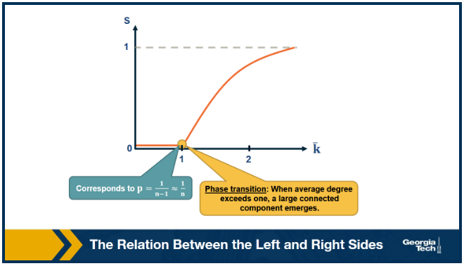
The visualization shows how S increases with the average node degree $\bar{k}$. Note how the LCC suddenly “explodes” when the average node degree is larger than 1. This is referred to as “phase transition”. A phase transition that we are all familiar with is what happens to water when its temperature reaches the freezing or boiling temperature: the macroscopic state changes abruptly from liquid to solid or gas. Something similar happens with G(n,p) when the average node degree exceeds the critical value $\bar{k}=1$: the network suddenly acquires a “giant connected component” that includes a large fraction of all network nodes.

Note that the critical point corresponds to a connection probability of $p = \frac{1}{n-1} \approx \frac{1}{n}$ because $\bar{k} = (n-1) \ast p$.

Here is another interesting question about the size of the LCC:

How Large should p (or $\bar{k}$ be such that the LCC covers all network nodes?

Our previous derivation we looked at the phase transition when $\bar{k} = 1$, which is just one area. Now suppose that S is the probability that a node does NOT connect to ANY node in the LCC: $$ (1-p)^{Sn} \approx (1-p)^n \text{ if } S \approx 1$$

The expected number of nodes not connecting to LCC:
$$ \overline{K_o} = n \cdot (1-p)^n = n(1-\frac{np}{n})^n \approx n \cdot e^{-np} $$ Recall that $(1 - \frac{x}{n})^n \approx e^{-x}$ when x << n

So we assume at this point of the derivation that the network is sparse (p << 1). If we set $\overline{k_o}$ to less than one node, we get that

$\begin{align} &= \implies n \cdot e^{-np} \le 1 \\ &= \implies -np \le ln(1/n) = -ln(n) \\ &= \implies p \ge \frac{ln(n)}{n} \\ &= \implies \bar{k} = np \ge ln(n) \end{align}$

Which means that when the average degree is higher than the natural logarithm of the network size ($\bar{k} > ln(n)$) we expect to have a single connected component.

Degree Correlations¶

In our discussion thus far we have assumed that node degrees are independent and uncorrelated.

ie Pr(degree(u)=k | degree(v)=k') Pr(degree(u)=k | u connects to some other node)$=q_k = p_k \cdot \frac{k}{\bar{k}}$

This is what's called a neutral network. When the degree of u does not depend on the degree k' of it's neighbour v.

In general networks have some correlation between neighbouring nodes. And they can be described as

Pr[k'|k] = Pr(a neighbor of a k-degree node has degree k')

The expected value of this distribution is referred to as the average nearest-neighbor degree $k_nn(k)$ of degree-k nodes.

$k_{nn}(k) \sum_{k'} k' \cdot P(k' | k)$

In a neutral network, we have already derived that $k_{nn}(k)$ is independent of k

recall that we derived $\large k_{nn}(k) = \bar{k} + \frac{\sigma_k^2}{\bar{k}} = \bar{k}_{nn}$

In most real networks, $k_nn(k)$ depends on k and it shows an increasing or decreasing trend with k.

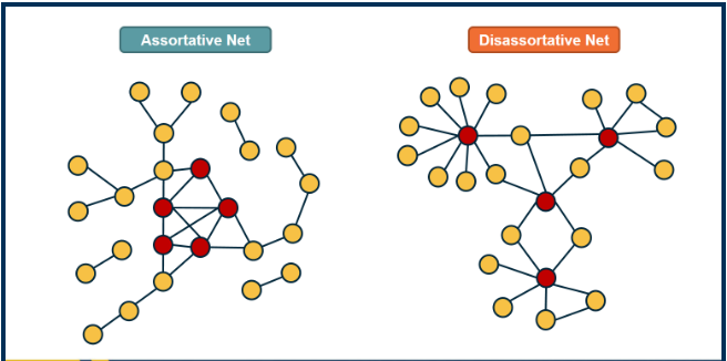
(left) is an example in which small degree nodes tend to connect with other small-degree nodes, (sim for high degree nodes)
(right) is a network in which small degree nodes tend to connect to high degree nodes.

A common approach to quantifying the degree is using the power law distribution to model the relationship between the average nearest neighbour degree $k_{nn}(k)$ and the degree k.

recall power law distribution: $k_{nn}(k) \approx a \cdot k^{\mu}$

If $\mu > 0$ we say that the network is Assortative: Higher degree nodes tend to have high-degree neighbours and lower-degree nodes tend to have lower-degree neighbors. Think of celebrities dating celebrities and loners dating other loners
if $\mu < 0$ we say that the network is Disassortative: higher degree nodes tend to have lower-degree neighbours. Think of a computer network in which high-degree aggrgation switches connect modstly to low-degree backbone routers.
if $\mu$ is statistically not significantly different from 0, then we say that the network is Neutral.

Suppose that instead of this power-law relation between $k_{nn}(k)$ and k we had used a linear statistical model. How would you quantify degree correlations in that case?

Hint: How would you apply Pearson's correlation metric to quantify the correlation between degrees of adjacent nodes?

Let's look at some degree correlation examples from the real world

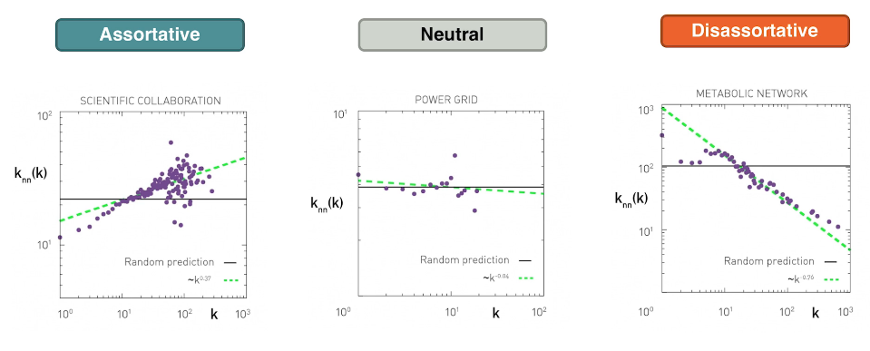
the first chart shows the degree of collaboration between groups of scientists. Two nodes, two scientists are connected if they have written at least one paper together. ie edges represent collaborative publications. Notice that the data is quite noisy especially when the degree K is more than about 70. The reason simply that we did not have a large enough sample of such nodes with large degrees. Nevertheless, we clearly see a positive correlation between the degree K and the degree of the nearest neighbour, on the y-axis. If we model the data with a power law relation, the exponent mu is approximately 0.37 in this case. We can use this value to quantify and compare the sort of activity of different networks when the estimate of mu is statistically significant.

The second chart represents a portion of the power grid in the united states here there is little evidence of correlation between a node k and the degree of it's nearest neighbour. So it is safe to assume that this network is what we call neutral.

The third network refers to a metabolic network where nodes here are metabolites. If two metabolites A and B appear in the opposite sides of the same chemical reaction in a biological cell, the data so a strong negative correlation in this case. But only if the nodes have degree 5, 10, or higher. If we model the data with power law relation, the exponent mu is approximately minus 0.76. This suggests that complex metabolites such as glucose, are either synthesised through a process called anabolism. Or broken down into, through a process called catabolism into a large number of simpler molecules such as carbon dioxide.

L3-Summary¶

The main objective of this lesson was to explore the notion of “degree distribution” for a given network. The degree distribution is probably the first thing you will want to see for any network you encounter from now on. It gives you a quantitative and concise description of the network’s connectivity in terms of average node degree, degree variability, common degree modes, presence of nodes with very high degrees, etc.

In this context, we also examined a number of related topics. First, the friendship paradox is an interesting example to illustrate the importance of degree variability. We also saw how the friendship paradox is applied in practice in vaccination strategies.

We also introduced G(n,p), which is a fundamental model of random graphs – and something that we will use extensively as a baseline network from now on. We explained why the degree distribution of G(n,p) networks can be approximated with the Poisson distribution, and analyzed mathematically the size of the largest connected component in such networks.

Obviously, the degree distribution does not tell the whole story about a network. For instance, we talked about networks with degree correlations. This is an important property that we cannot infer just by looking at the degree distribution. Instead, it requires us to think about the probability that two nodes are connected as a function of their degrees.

We will return to all of these concepts and refine them later in the course.

L3 Appendix¶

ref: http://networksciencebook.com/chapter/3#introduction3

Random Network Model¶

Most real world networks do not fit into nice graphs with well known patterns like a lattice. Random network theory embraces the idea of randomness by contructing and characterizing networks that are truly random. The challenge with random models is that although they appear as relatively simple objects with nodes and edges, it is their complexity in modelling a real world that makes the statistical in nature. A simple example might be the power grid or the world wide web. Every day new power lines are being constructed and destructed. A new blogger may have just a launched a new website to preach upon.

Nutshell A random network consists of N nodes where each node pair is connected with probability p.

There are two main types of Random Network Models:

G(N, L) Model: N labeled nodes are connected with L randomly placed links. Erdős and Rényi used this definition in their string of papers on random networks. A G(N,L) model has a fixed number of links
G(N, p) Model: Each pair of N labeled nodes is connected with probability p, a model introduced by Gilbert. A G(N,p) model has a fixed probabilty p that 2 nodes are connected

We will focus exclusively on G(N,p).

Should you wish to create a random network the procedure is rather simple:

start with N isolated nodes
for i = 1 -> N(N-1) 
    - Select a node pair, say a,b
    - generate a random number k b/w 0 and 1 
    - if k > p then add an edge from a to b

Number of Links¶

The expected number of links in a random graph is given by

$\large \langle L \rangle = \sum_{L=0}^{N(N-1)/2} L_{p_L} = p \frac{N(N-1)}{2}$

The average degree of a random network is given by

$\large \langle k \rangle = \frac{2 \langle L \rangle}{N} = p(N-1)$

observations

increasing p leads to a denser network
- the avg number of links increases linearly from 0 to $L_{max}$
- the avg degree of a node increases from 0 to N-1

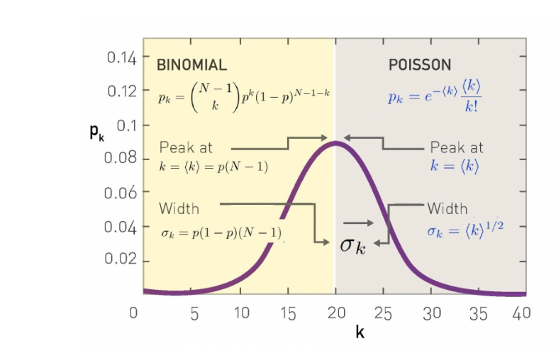
Incidentally you may notice a striking similarlity to the binomial distribution, this is not a coincidence it is in fact binomially distributed. You may also wish to recall that in practice the binomial distribution is often approximated by the poisson distribution

Number of Degrees¶

The degree distribution of a random network, ie the probability that a node i has exactly k links is given by the product of

The probability that k of its links are present, $p^k$
The probability that the remaining (N-1-k) links are missing, or $(1-p)^{N-1-k}$
The number of ways to choose k links from N-1 possible links, ${N-1} \choose k$

Put them together and you get:

$p_k = {{N-1} \choose k} p^k (1-p)^{N-1-k}$
- which is the binomial
but to approximate $p_k = e^{-\bar{k}} \frac{\bar{k}^k}{k!}$
- which is the poisson
- note that the 1/k! term significantly decreases the chances of observing large degree nodes
Both distributions have a peak around ‹k›. If we increase p the network becomes denser, increasing ‹k› and moving the peak to the right.
The width of the distribution (dispersion) is also controlled by p or ‹k›. The denser the network, the wider is the distribution, hence the larger are the differences in the degrees.

Unless otherwise stated we will always be using the poisson in terms of $\bar{k}$

Evolution of a Random Network¶

Imagine modelling a cocktail party as a network, You begin with N nodes and as they walk around during the night they introduce themselves and form connections. This is an example of the G(N,p) model where p is the probability of a connection. At the start of the night p is quite small and as the night improves p increases until it reaches some maximum. At this point everyone is connected to everyone.

p=0, then $\bar{k}=0$, all nodes are isolated
- t/f the largest component $N_G$ is of size 1
- and $N_G / N \rightarrow 0$ for a large N
p=0, then $\bar{k}=N-1$, network is a complete graph and
- all nodes belong to a single component
- t/f $N_G = 1$ and $N_G / N = 1$

L4 : Random v Real Graphs & Power Law Networks¶

L4 Intro¶

Learning Objectives:

See examples of real networks with highly skewed degree distributions
Understand the math of power-law distributions and the concept of “scale-free” networks
Learn about models that can generate networks with power-law degree distribution
Explain the practical significance of power-law degree distributions through case studies

Readings:

sections 4.1, 4.2, 4.3, 4.4., 4.7, 4.8, 4.12
sections 5.1, 5.2, 5.3

Scientists used to think that real world network models could be modelled using the Erdős–Rényi (ER) Graph. Such networks follow a binomial distribution. And you may recall that the poisson is often used to approximate this.

Back in the 1990s researchers observed that real networks are actually quite different. Their degree distribution were highly skewed. For such phenomena it was determined that the power-law distribution was much more fitting.

Take note:

Poisson is clearly a very bad model because it cannot capture the large variability and skewness of the degree distribution
Plots shown in log-log scale with a degree distribution that decreases roughly as straight lines.
- This means the probability a node has degree k drops as a power law of $k: p_k \sim k^{-\alpha}$
- The slope of that straight line corresponds to the exponent of the power law $\alpha$

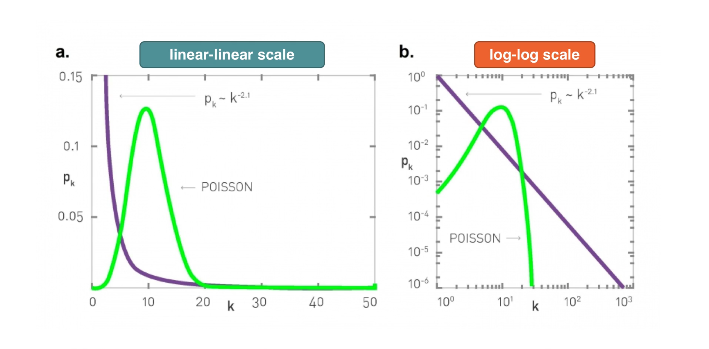
Here are the two distributions in both linear-linear and log-log scales. Poisson distribution has an average degree of 11 here, while the power-law distribution has a lowered average degree set to 3 and the exponent to 2.1.

The linear-linear plot shows that almost bell-shaped form of the Poisson distribution centered around its mean. The power-law distribution on the other hand is not centered around the specific value. The major difference between the two distributions becomes clear in log-log scale. We see that the Poisson distribution cannot produce values that are much larger than its average.

In this example, the maximum value of the Poisson distribution is roughly 30, about 3 times larger than the mean. The power-law distribution extends over three orders of magnitude. And there is a non-negligible probability that we get values that are much greater than its mean.

Power Law¶

Power Law Distribution

$\large p_k = ck^{-\alpha}$
- probability that the degree of a node is equal to a positive integer k is proportional to $k^{-\alpha}$ for $\alpha=0$
- coefficient c is chosen s.t. the sum of all degree probabilities is 1 for a given $\alpha$
- and a given min degree $k_{min}$

if you think of the power law distribution as a continuous density and integrate you'll find that

$\large c = (\alpha - 1) k_{min}^{\alpha-1}$
just replace summation with the integral

Hence the power-law distribution can be stated as

$\large \frac{\alpha-1}{k_{min}} (\frac{k}{k_{min}})^{-\alpha} $

With a Complementary CDF as

$\large Pr[degree \ge k] = (\frac{k}{k_{min}})^{-(\alpha - 1)} $
note the exponent here is $-(\alpha - 1)$

A Mean as

$\large E[k^m] = \sum_{k_{min}}^{\infty} k^m p_k = c \sum_{k_{min}}^{\infty} k^{m-\alpha} $
where c is the same as above
this can also be integrate to see that this will
- converge to $\infty$ if $m-\alpha+1 \ge 0$
- t/f finite and integrable when $m \lt \alpha-1 $

In most real-world networks $\alpha$ is estimated to be between 2 and 3.

Can you think of a network with n nodes in which all nodes have about the same in-degree but the out-degrees are highly skewed?

In practice, the degree distribution may not follow an ideal power-law distribution throughout the entire range of degrees. In other words, the empirical degree distribution may not be a perfect straight-line when plotted in log-log scale.

For lower values of k we observe a low-degree saturation that decreases the probability of seeing low-degree nodes compared to an ideal power-law. If this saturation effect takes place for nodes say less than $k_{sat}$ then we can modify our power law expression as : $(k + k_{sat})^{-\alpha}$
- this will effectively shift the lower degree nodes higher
- while leaving the higher degree nodes relatively unchanged in distribution
an alternative approach for low-degree saturation is to rescale the distribution
For higher values of k we often trim or cut the higher values. Reason being is that the real world often contains constraints that affect the maximum of the degree nodes.

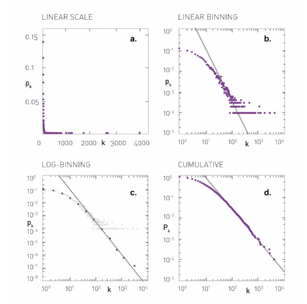
Plotting a Degree Distributions: A degree distribution of the form pk ~ (k + k0)-γ, with k0=10 and γ=2.5, plotted using the four procedures described in the text:

Linear Scale, Linear Binning. It is impossible to see the distribution on a lin-lin scale. This is the reason why we always use log-log plot for scale-free networks.
Log-Log Scale, Linear Binning. Now the tail of the distribution is visible but there is a plateau in the high-k regime, a consequence of linear binning.
Log-Log Scale, Log-Binning. With log-binning the plateau dissappears and the scaling extends into the high-k regime. For reference we show as light grey the data of (b) with linear binning.
Log-Log Scale, Cumulative: The cumulative degree distribution shown on a log-log plot.
- This is the best approach because we do not need to determine an appropriate sequence of bin-widths. Please note however that the slope of the C-CDF is not the same as the slope of the degree distribution. In this example, $\alpha=2.5$ and so the exponent of the C-CDF is 1.5.

Scale Free Property¶

Recall that the Normal distribution describes quite accurately many random variables (due to the Central Limit Theorem), and that according to that distribution 99.8% of the data are expected to fall within 3 standard deviations from the average. this is true for all distributions with exponentially fast decreasing tails, which includes the Poisson distribution and many others. In networks that have such degree distributions, the average degree represents the “typical scale” of the network, in terms of the number of connections per node.

On the other hand, a power-law degree distribution with exponent $2 < \alpha < 3$ has finite mean but infinite variance (any higher moments, such as skewness are also infinite). The infinite variance of this statistical distribution means that we cannot expect the data to fall close to the mean. On the contrary, the mean (the average node degree in our case) can be a rather uninformative statistic in the sense that a large fraction of values can be lower than the mean, and that many values can be much higher than the mean (see purple distribution at the visualization).

For this reason, people often refer to power-law networks as “scale-free”, in the sense that the node degree of such networks does not have a “typical scale”. In the rest of this course, we prefer to use the term “power-law networks” because it is more precise.

Basically a scale free network is just a power-law network.

MaxDegree - Power Law Networks¶

Let's now consider the maximum degree in a power-law distribution as compared to that of say an exponential distribution. We choose exponential for it's convenience as well as the fact that it decays less rapidly than the poisson used to model a G(n,p) network.

recall that an exponential distribution is given by $p_k = ce^{-\lambda k}$

where k is the degree
$1/\lambda$ is the avg degree
and c is a normalization constant

In a network where the min degree is k_min >= 0 and with 1/lambda > kmin the parameter c should be equal to $\lambda e^{\lambda k{min}}$ hence

$\large p_k = \lambda e^{\lambda k_{min}} e^{-\lambda k} $

furthermore suppose that the max degree k_max is unique and to P[degree(N_i) = k_max] = 1/n

then $\large \int_{k_{max}}^{\infty} p_k dk = 1/n$

put these together and integrate to get

k_max = k_min + ln(n)/lambda
This means that the maximum degree increases very slowly (logarithmically) with the network size n, when the degree distribution decays exponentially fast with k

Repeating this derivation for a power-law network yields

$\large k_{max} = k_{min} n^{1/(\alpha - 1)}$
This means that the max degree in a power law network increases as a power law of the network size n. for $\alpha=3$ the max degree increases with the square root of n. In the more extreme case $\alpha=2$ the max degree increases linearly with n!

for example consider a network with 1M nodes, and an avg deg k_avg = 3. if the network is exponential then the max degree is around 10 which is not much larger than the avg degree. However, if the network follows a power law distribution with alpha=2.5 then the max degree is about 10,000!!

This is actually not that crazy. In the real world networks often have hubs that have super high degree's. Airports are a great example as this as many small airports get very few flights. Larger airports serve as connection points and as a base for airline companies. These are hubs with higher than avg degrees

Failures and Attacks¶

first let's define some terms

random failure: some fraction, f, of randomly selected nodes are removed from the system
Targeted attack: Fraction, f, of nodes with highest degree are removed from the system

As it turns out Power-Law networks are quite robust in the first case, but completely disintegrate in the 2nd. Similarly Poisson networks don't have hubs and can survive the second case much better.

Degree Preservation¶

It is often the case in network analysis that we have a network G with a property P. P can be one of the above properties or something else from your imagination. How can we verify if P holds for different degree distributions??

Type 1: Randomize the network G without modifying any node's degree, ie degree preservation. Type 2: fully randomized Create another ensemble of randomized networks that do not have the same degree distribution with G but still maintain the same number of nodes and edges.

If P of G is present in one of the types but not the other then we can be confident it is a consequence of that target. In general we want to know if P holds under degree preservation.

Methodology

Full Randomization
- pick an edge (a,b) and randomly replace b with some other node
- this will certainly impact the degree distribution
- may disconnect nodes, highly unlikely to have hubs
Degree preservation
- pick two edges at random (s1,t1) and (s2,t2)
- rewire to (s1,t2) and (s2,t1)
- repeat until each node is rewired at least once

Power Law Avg Degree¶

Recall for a neutral network (0 correlation between neighbours)

$\bar{k_n} = \bar{k} + \sigma^2 / \bar{k} $
is the avg neighbour degree

However, we've shown that PL networks also have hubs that increase the avg degree.

Configuration Model (Synthetic)¶

These are networks we create in order to model a real world network with a given distribution.

A general way to create synthetic networks with a specified degree distribution $p_k$ is the “configuration model”. The inputs to this model is

a) the desired number of nodes n, and
b) the degree ki of each node i

The collection of all degrees specifies the degree distribution of the synthetic network.

The configuration model starts by creating the n nodes: node i has ki available “edge stubs”. Then, we keep selecting randomly two available stubs and connect them together with an edge, until there are no available stubs. The process is guaranteed to cover all stubs as long as the sum of all node degrees is even.

The configuration model process is random and so it creates different networks each time, allowing us to produce an ensemble of networks with the given degree distribution. Additionally, note that the constructed edges may form self-loops (connecting a node to itself) or multi-edges (connecting the same pair of nodes multiple times).

Preferential Attachment Model¶

The configuration model above describes the creation of a model, but it lacks any guidance on how to grow a network. ie how to add nodes such that the network becomes a PL distributed. This is where the preferential model steps in

The preferential model grows a network by one node in each time step. Thus after t steps we have t nodes. Each time a node is added it is connected to m existing nodes. m is a constant throughout the growth

Let K_i(t) be the degree of node i at time t

then the probability that the new node will connect to node i is given by
$\large \prod_i(t) = \frac{k_i(t)}{\sum_j^t k_j(t)} = \frac{k_i(t)}{2mt}$

This tells us that

As the network grows over time and new nodes are more likely to connect to nodes with higher degrees
the rich get richer effect
- hub nodes tend to attract more new connections as nodes are added

The preferential model will produce PL networks with an $\alpha=3$

How might this be modifed to produce a PL network with alpha between 2 & 3?

Link Selection Model

Suppose that each time we introduce a new node, we select a random link and the new node connects to one of the two end-points of that link (randomly chosen). In other words, the new node connects to a randomly selected edge-stub

In this model, the probability that the new node connects to a node of degree k is proportional to k (because the node of degree-k has k stubs). But this is exactly the same condition with the preferential attachment model: a linear relation between the degree k of an existing node and the probability that the new node connects to that existing node of degree-k.

Link selection model is just a variant of preferential attachment and it also produces power-law degree distribution with exponent $\alpha=3$

Power Law in Practice¶

let us consider the case of networks of sexual partners. There are several diseases that spread through sexual intercourse, including HIV-AIDS, syphilis or gonorrhea.  The degree distribution in such networks relates to the number of sexual partners of each individual

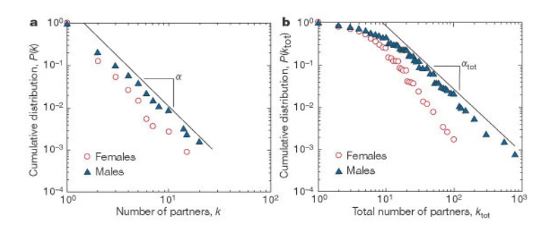
The plot at the left is the C–CDF for the number of partners of each individual during the last 12 months, shown separately for men and women. Note that the distributions drop roughly linearly in the log-log scale plot, suggesting the presence of a power-law distribution (at least in the range from 2 to 20). 

The plot at the right is the corresponding C-CDF but this time for the entire lifetime of each individual. As expected, the range of the distribution now extends to a wider range (up to 100 partners for women and 1000 for men). Note the low-degree saturation effect we discussed earlier in this lesson, especially for less than 10 partners.

L5 Network Paths, Clustering, Small World Property¶

Learning Objectives:

Introduce the “network efficiency” concept and define the relevant quantitative metrics
Introduce the “network clustering” concept and define the relevant quantitative metrics
Explain differences between “small-world” networks and random/regular/power-law networks
Introduce the "network motifs" concept and define the relevant quantitative metrics
Explain the significance of “small-world” networks through case studies

Readings:

Basabasi: 3.8, 3.9, 5.10

Clustering Co-Efficient¶

Suppose three nodes in a social network are connected. ie they form a triangular cycle. How would we quantify such a cluster? For this we use the clustering co-officent. For a node i this is defined as the fraction of it's neighbours that are also connected.

Mathematically

for an undirected, unweighted network
$\large C_i = \frac{1/2 \sum_{jm} A_{i,j} A_{j,m} A_{m,i} }{ k_i(k_i - 1)/2}$
$\large = \frac{\sum_{jm} A_{i,j} A_{j,m} A_{m,i} }{ k_i(k_i - 1)}$
where denominator is the number of distinct neighbour pairs of node-i
and the numerator is the number of pairs that form triangles
of course A refers to the adjacency matrix
This is not defined for nodes with degree 0

three examples in which node-i is the purple node

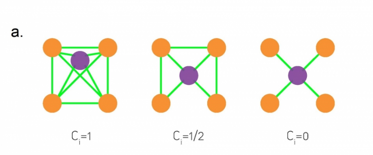
However, in general we will look at the avg clustering co-efficient across the entire network. Typically there is a decreasing trend in C(k) as k increases, suggesting that it becomes less likely to find densely interconnected clusters of many nodes compared to clusters of fewer nodes.

To quantify the degree of clustering across an entire network we have two options

The average clustering co-efficient, which isn't great
Transitivity (aka global clustering co-efficient). This is defined as the fraction of the connected triplets of nodes that form triangles.

T = (3 x Number of triangles) / (number of triplets)
where a triplet is defined as an ordered set of three nodes, such ABC, that are connected, ie A-B and B-C.
a fully connected triangle of three nodes ABC is three triplets: ABC, BCA, CAB
An open triplet would be say BA & BC but where A doesn't connect to C

Transitivity and the Average Clustering Coefficient are two different metrics. They may often be close but there are also some extreme cases in which the two metrics give very different answers. To see that consider a network in which two nodes A and B are connected to each other as well as to every other node. There are no other links. The total number of nodes is n. What would be the transitivity and average clustering coefficient in this case (you can simplify by assuming that n is quite large)?

In weighted networks¶

First we define the strength as the sum of all weights of the node's connections

ie $s_i = \sum_j A_{i,j} w_{i,j}$

Then we define the clustering co-efficient of node i as

$\large C_w(i) = \frac{1}{s_i(k_i-1)} \sum_{j,h} \frac{w_{i,j} + w_{j,h}}{2} A_{i,j} A_{i,h} A_{j,h}$
the first term is just a normalizing factor
the product of three adjacency elements is 1 iff i,j,h form a triangle

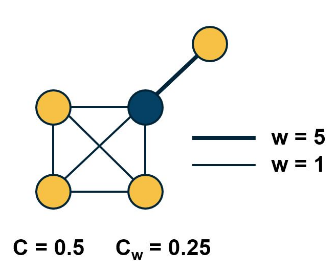
The visualization above show the unweighted and weighted clustering coefficient values for the darker node. That node has a stronger connection with a node that does not belong to the cluster of nodes at the lower-left side. This is why the weighted clustering coefficient is lower than the unweighted.

Network Types: G(n,P) & Regular¶

G(n,P)

Recall that any two nodes in an ER model are connected with the same probability p. Hence the probability of a triplet forming a triangle is also p. and the exp value of the clustering co-efficient for any node with more than one connection is p as well, and the transitivity is p too.

In G(n,p) the avg degree is $\bar{k}=p(n-1)$, t/f if the avg degree remains constant the p should drop inversely proportional with n as network size grows. And we will see a decreasing tren b/w the clustering co-efficient and the network size.

The G(n,p) model predicts negligible clustering, especially for large and sparse networks. On the contrary, real-world networks have a much higher clustering coefficient than G(n,p) and its magnitude does not seem to depend on the network size

Regular Networks

In regular networks we will typically see locally clustered topology. The exact value of the clustering coefficient depends on the specific network type but in general, it is fair to say that “regular networks have strong clustering”. Further, the clustering coefficient of regular networks is typically independent of their size.

Consider a circle graph where every node is connected to an even number c of it's nearest neighbours. For a ring network c=2 and has 0 clustering. However for higher values of c transitivity is: T=( 3(c-2) / 4(c-1) ). Which as you can image will converge to 3/4 as c grows large.

Other Metrics

Small world networks depend on two concepts

How clustered the network is
how short the paths between network nodes are

Avg Shortest Path Length / Characterisitic Path Length

$\large L = \frac{2}{n(n-1)} \sum_{i<j} d_{i,j}$

Efficiency - aka harmonic mean

$\large E \frac{2}{n(n-1)} \sum_{i<j} \frac{1}{d_{i,j}}$

Diameter

$\large D = max_{i<j} d_{i,j}$

A more informative description is the distribution of the shortest-path lengths across all distinct node pairs, as shown in the visualizations below.

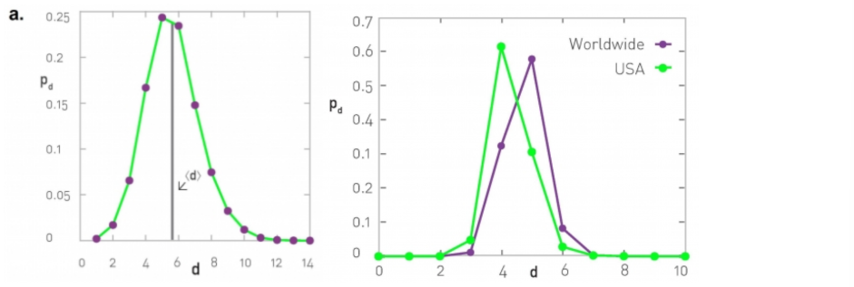
At left, the corresponding network is the largest connected component of the protein-protein interaction of yeast (2,018 nodes and 2,930 edges, the largest connected component include 81% of the nodes). The characteristic path length (CPL) is 5.61 while the diameter is 14 hops.

At right, the network is based on the friendship connections of Facebook users (all pairs of Facebook users worldwide and within the US only). The CPL is between 4 and 5, depending on the network.

G(n,p) - Other metrics¶

Let's look back at the G(N,p) model in light of the above metrics.

Suppose $\bar{k}=p(n-1) > 1$, so that the network has a giant connected component

We start at node i
in just 1 step we expect to visit $\bar{k}$ nodes
- in 2 step we expect to visit $\bar{k}^2$ nodes
- after s hops we expect to visit $\bar{k}^s$
but the total number of nodes is n so we expect to visit all of them with the maximum number of hops
- of course this is D the diameter
so $n \approx \bar{k}^D$
we can solve for D to get
$D \approx \frac{\ln n }{\ln \bar{k}}$
- this expression is a very rough approximation, it shows something remarkable: in a random network, even the longest shortest—paths are expected to grow very slowly (i.e., logarithmically) with the size of the network.

( Aside: Suppose our network is the population of earth? Around 7B people. Futhermore suppose each person knows 64 people or more. Then the shortest path between any 2 people would be around 5.4. ) This is where the 6-degrees of seperation comes from

Consideration
When working with sparse and dense networks there are some special considerations

for very sparse networks as k approaches 1 from above the diameter is expected to be
- $D \approx 3 \frac{\ln n }{\ln \bar{k}}$
- which is 3 times larger than above
for very dense networks the diameter is expected to be
- $D \approx \frac{\ln n }{\ln \bar{k}} + \frac{2 \ln n }{\bar{k}} + \ln n \frac{\ln \bar{k}}{(\bar{k})^2}$

Note that in both cases, the diameter is still increasing with the logarithm of the network size. So, the main qualitative conclusion remains what we stated in the previous page, i.e., the diameter of G(n,p) networks increases very slowly (logarithmically) with the number of nodes – and so the CPL cannot increase faster than that either.

Lattice Networks

In one-dim lattices, each node has 2 neighbors, and the lattice is a line network of n nodes. So the diameter increases linearly with n.
In two dimensions, each node has 4 neighbors, and the lattice is a square with nodes on each side -- so the diameter increases as O($n^{1/2}$)
Similarly, in three dimensions each node has 8 neighbors, and the diameter grows as O($n^{1/3}$) - and so on in higher dimensions.

This suggests that in lattice networks the diameter grows as a power-law of the network size – this grows much faster than a logarithmic function.

L5B Small Worlds¶

A Small-World network is one that satisifes the following two characterisitics

1-The clustering coefficient is much larger than that of the random G(N,p) network
2-The CPL (Avg SPL) of the network is not significantly greater than that of the random G(N,p)
these conditions generally depend on some type of significance level. of the corresponding hypothesis tests.

Networks we often see in practice have the following two properties,

they have strong clustering similar to that of lattice networks with the same average degree,
second, they have short paths similar to the CPL and diameter we see in random Erdos-Renyi, ER, networks for the same n,P

They are small in the sense that the shortest paths between nodes increase only modestly with a size of the network. Modestly means logarithmically or even slower. At the same time, small-world networks are not randomly formed. On the contrary, the nodes form clusters of interconnected triangles, similar to what we see in social groups, such as families, groups of friends, or larger organizations of people.

Watts Strogatz Model¶

The WS model is a Random graph model that produces a network with a small-world property.

The model starts with a regular network with the desired number of nodes and average degree. The topology of the regular network is often a ring graph. With a small probability p, we select an edge and reassign one of its two stubs to a randomly chosen node as you see here. You may wonder, why do we expect that a small fraction of randomized edges will have any significant effect on the properties of this network. It turns out that even if this rewiring probability p is quite small, the randomized edges provides shortcuts that reduce the length of the shortest paths between node pairs. As we will see next, even a small number of such shortcuts, meaning a rewiring probability p close to 1% is sufficient to reduce the characteristic path length and the diameter down to the same level with a corresponding random G(N,p) network.

At the same time, very wired network is still highly clustered at the same level with the regular network we started from as long as p, of course, is quite small. If this rewiring probability p was set to one, we would end up with a random GNP graph, which is what we see at the right. This network would have even shorter path, but it would not have any significant clustering.

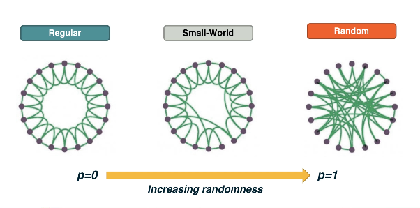
You may wonder, is the Watts-Strogatz Model able to produce networks with a power load degree distribution? The answer is no. The degree distribution of that model depends on the rewiring probability p. If p is close to 0, most nodes have the same degree. As p approaches 1, we get the Poisson degree distribution of a random graph. In every way, the resulting degree distribution is not sufficiently skewed towards higher values. It cannot be mathematically modeled as a power load and we do not see hubs.

In summary, even though the Watts-Strogatz Model was a great first step in discovering two important properties of real-world networks, clustering and short paths, it is not a model that can construct realistic networks because it does not capture the degree distribution of many real-world networks.

Preferential Model Revisited¶

Networks are generated with the PA model, with m=2 links for every new node. Note that the clustering coefficient is significantly higher than that of random G(N,p) random graphs of the same size and density (p=m/(N-1)). It turns out (even though we will not prove it here) that the average clustering coefficient of a PA network scales as $(ln N)^2 / N$ this is much larger than the corresponding clustering coefficient in G(N,p), which is O(1/N).

clustering coefficient

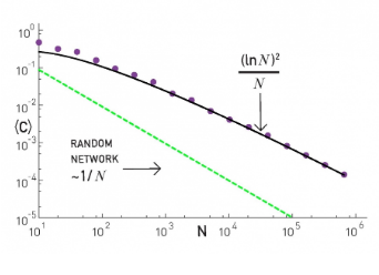
This also means that the clustering coefficient of PA networks decreases with the network size N. This is not what we have seen in practice (see figure at the right). In most real-world networks, the clustering coefficient does not reduce significantly at least as the network grows. Thus, even though the PA model produces significant clustering relative to random networks, it does not produce the clustering structure we see in real-world networks.

Length of shortest paths in PA Model
It also turns out that the CPL in PA Networks scales even slower than G(N,p) random graphs. In particular, an approximate expression for CPL in a PA network is O(ln N / ln(ln(N))) which is sublogarithmic

Directed Networks¶

13 different types of connection patterns between three weakly connected network nodes. Note that each of the 13 patterns is distinct when we consider the directionality of the edges.

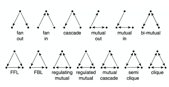
Each of these patterns is also given a name (e.g., FeedForward Loop or FFL). Instead of using the word “pattern”, we will be referring to such small subgraph types as network motifs.

Statistical Tests for Network Motifs

Suppose we are given a 16-node network G, and we want to examine if the FFL network motif appears too frequently. How would we answer this question?

First, we need to count how many distinct instances of the FFL motif appear in G. One way to do so is to go through each node u that has at least two outgoing edges. For all distinct pairs of nodes v and w that u connects to uni-directionally, we then check whether v and w are also connected with a uni-directional edge. If that is the case (u,v,w) is an FFL instance. Suppose that the count of all FFL instances in the network G is m(G).

We then ask: how many times would the FFL motif take place in a randomly generated network $G_r$ that a) has the same number of nodes with G, and b) each node u in $G_r$ has the same in-degree and out-degree with the corresponding node u in G? One way to create is to start from G and then randomly rewire it as follows:

Pick a random pair of edges of (u,v) and (w,z)
Rewire them to form two new edges (u,z) and (w,v)
Repeat the previous two steps a large number of times relative to the number of edges in G.

Each previous rewiring process generates a network $G_r$ that preserves the in-degree and out-degree of every node in G. We can now count the number of FFL instances in $G_r$ – let us call this count m($G_r$).

The previous process can be repeated for many randomly rewired networks $G_r$ (say 1000 of them). This will give us an ensemble of networks. We can use the counts m($G_r$) to form an empirical distribution of the number of FFL instances that would be expected by chance in networks that have the same number of nodes and the same in-degree and out-degree sequences as G.

We can then compare the count m($G_r$) of the given network with the previous empirical distribution to estimate the probability with which the random variable m($G_r$) is larger than m($G$) in the ensemble of randomized networks. If that probability is very small (say less than 1%) we can have a 99% statistical confidence that the FFL motif is much more common in G than expected by chance.

Similarly, if the probability with which the random variable m($G_r$) is smaller than m($G$) is less than 1%, we can have 99% confidence that the FFL motif is much less common in G than expected by chance. The magnitude of m($G$) relative to the average plus (or minus) a standard deviation of the distribution m($G_r$) is also useful in quantifying how common a network motif is.

The method we described here is only a special case of the general bootstrapping method in statistics.

L6 Centrality and Network Code Metrics¶

Objectives:

Understand the problem of finding individually important nodes/edges or groups of important nodes/edges
Define and analyze common centrality metrics
Define and analyze common “network core” metrics
Learn how to apply centrality metrics and core identification algorithms through case studies

Centrality¶

Degree and Strength Centrality
This is the simplest of all the measures. It is simply the number of connections it has. The more it has the more important it is. Effectively degree centrality is just the degree.

For a weighted network, we use the strength of the node. Strength is defined as the sum of weights of all edges of that node.

For a directed network we seperate the in/out degree.

Degree and strength measure are far from perfect. For ex the only node between two large clusters is important but may have a rather low degree relative to the degree distribution. It's also easy to manipulate. Back in the early days of the internet sites would manipulate google results by boosting their page's centrality. This was done by creating pages that link to their page.

Eigenvector Centrality

Eigenvector centrality (also called eigencentrality or prestige score[1]) is a measure of the influence of a node in a network. Relative scores are assigned to all nodes in the network based on the concept that connections to high-scoring nodes contribute more to the score of the node in question than equal connections to low-scoring nodes. A high eigenvector score means that a node is connected to many nodes who themselves have high scores.

The idea here is that a node is more central when it's neighbours are also more central.This is defined using the adjacency matrix A as follows

for undirected network: $v_i = \frac{1}{\lambda} \sum_i A_{i,j} v_j$ ($v_j$ is the centrality of node j)
since $\frac{1}{\lambda}$ is a normalizing constant
and $v_j$ can be written as a one dimensional vector
we can summarize this as $\lambda v = Av $

This may look familiar to many of you. It's the eigenvector definition of matrix A. $\lambda$ is the corresponding eigenvalue for eigenvector v. and we refer to this centrality metric as "eigenvector centrality".

You may also recall that there are eigenvectors with negative elements

The Katz Centrality

Katz centrality is variation of the eigenvector for directed networks. It takes the previous measure as it's base and adds a small centrality constant $\beta$ to all nodes. part of the reason for this is that the eigenvector measure can be zero for some nodes despite having both in and out degrees.

Katz: $v_i = \beta + \frac{1}{\lambda} \sum_i A_{i,j} v_j$
where the summation is over all nodes j that connect i

We can also take $\beta = 1$ since we only care about the magnitude of the centrality values.
Now we can rewrite the matrix eqn as follows

$v = (I - \frac{1}{\lambda} A)^{-1} . 1$ where 1 is just a nx1 matrix of ones
$\lambda$ controls the relative magnitude b/w the constant centrality $\beta$ assigned to each node and the centrality that each node derives from it's neighbours. if $\lambda$ is very large then the first term dominates and all nodes will have similar centrality. However, if $\lambda$ is small then the katz centralities may diverge. ( incidentally this is because the determinant of $(I - \frac{1}{\lambda})$ is 0, which in turn happens when $\lambda$ is equal to some eigenvalue of A.
To prevent this $\lambda$ is often constrained to be larger than the max eigenvalue of A.

PageRank Centrality

PageRank is the name given to the algorithm created by the founders of Google, Larry Page and Sergey Brin. At it's core is the Katz Centrality measure we described in the previous section.

It can be described as follows:

If a node j points to a node i (and thus $A_{i,j} = 1$) and node j has $k_{j,out}$ outgoing connections, then the centrality of node j should be split among it's $k_{j,out}$ neighbours. Another way to think of this is that out-going connections share in the wealth of the node j, they do not simply inherit. In the inheritance approach of Katz all outgoing neighbours would effectively get the same centrality as j
$v_i = \beta + \frac{1}{\lambda} \sum_i A_{i,j} v_j \frac{v_j}{k_{j,out}} $
where the summation is over all nodes j that point to i ( thus $k_{j,out}$ is non-zero )

We can also write this in matrix notation as $v = (I - \frac{1}{\lambda} A D)^{-1} . 1$. Where D is a diagonal n by n matrix in which the j'th element is $1/k_{j,out}$. In undirected networks we can replace the connections with a pair of directed edges to achieve this. In practice the computation of both Katz ans PageRank is usually done using iterative numerical methods. Typical values for $1/\lambda$ is 0.85 and for $\beta$ is $(1-1/\lambda)/n$. if $\lambda$ is too low it may fail to converge.

Closeness Centrality

These metrics focus on paths instead of nodes. In a manner, centrality in the path context, is a measure of how good a path is to the rest of the network. How many paths traverse a node would raise it's importance and centrality.

Closeness Centrality: is based on the length of the shortest path between nodes and i and j, and is denoted $d_{i,j}$. The closeness centrality of node i is defined as the inverse of the avg shortest path length $d_{i,j}$, across all nodes j&i connect to.

$v_i = \frac{n-1}{\sum_j d_{i,j}}$
where j is any node in the same connected component with i,
and n is the number of nodes in that connected component (including i).
range of closeness centrality will fall between 0 and 1

One shortcoming is that it focuses on nodes in the same connected component as i. This means that an isolated cluster of nodes can have high closeness centrality values even though those nodes are not connected to the rest of the network

Harmonic Centrality

This is a slightly improved version of the Closeness metric.

$v_i = \sum_{j \ne i} \frac{n-1}{d_{i,j}}$

Here we sum over all nodes, this will take into account all the nodes that can't be reached from j. Nodes that can't be reached have an infinite length, thus The term 1/d_i,j is taken as 0.

Betweenness Centrality

This is based on the shortest path idea, the "Shortest-Path betweenness centrality". Consider any 2 nodes s and t in the same connected component. We can define the shortest path b/w them as $n_{s,t}$, furthermore define $n_{s,t}(i)$ as the shortest path b/w s and t going through node i, i cannot be either s or t.

Then $\large v_i = \sum_{s,t \ne i} \frac{n_{s,t}(i)}{n_{s,t}}$
if s and t are the same take $n_{s,t}=1$

Note that node E, in the visualization, has higher betweenness centrality than node C – even though the two nodes have the same closeness centrality (and node C has higher eigenvector centrality than node E). The reason is that node E is the only “bridge” between nodes F and G and the rest of the network. For weighted networks, where the (non-negative) weight represents the cost of an edge, the shortest-paths can be computed using Dijkstra’s algorithm for weighted networks.

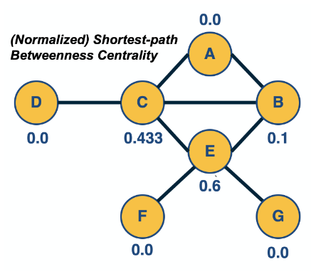
There are many variants of the betweenness centrality metric, depending on what kind of paths we use. One such variant is the flow betweenness centrality in which we compute the max-flow from any source node s to any target node t – and then replace the fraction $\frac{n_{s,t}(i)}{n_{s,t}}$ with the fraction of the max-flow that traverses node i.

Yet another variant is the random-walk betweenness centrality, which considers the number of random walks from node-s to node-t that traverse node-i.

Edge Centrality

In this case, we are interested in the centrality of edges, rather than nodes. For example, suppose you are given a communication network and you want to rank links based on how many routes they carry.

One such metric is the edge betweenness centrality. The definition is the same as for node betweenness centrality – but instead of considering the fraction of paths that traverse a node i, we consider the fraction of that traverse an edge (i,j). These paths can be shortest-paths or any other well-defined set of paths, as we discussed on the previous page.

Another way to define the centrality of an edge is to quantify the impact of its removal. For instance, one could measure the increase in the Characteristic Path Length after removing edge (i,j) – the higher that CPL increase is, the more important that edge is for the network.

DAG - Path Centrality

In directed acyclic graphs (DAGs), we can consider all paths from the set of sources to the set of targets. The visualization above shows a DAG with three sources (orange nodes) and four targets (blue nodes). Each source-target path (ST-path) represents one “dependency chain” through which that target depends on the corresponding source.

The path centrality of a node (including sources or targets) is defined as the total number of source-target paths that traverse that node.

It can be easily shown that the path centrality of node-i is the product of the number of paths from all sources to node-i, times the number of paths from node-i to all targets. The former term can be thought of as the “complexity” of node-i, while the second term can be thought of as the “generality” of node-i.

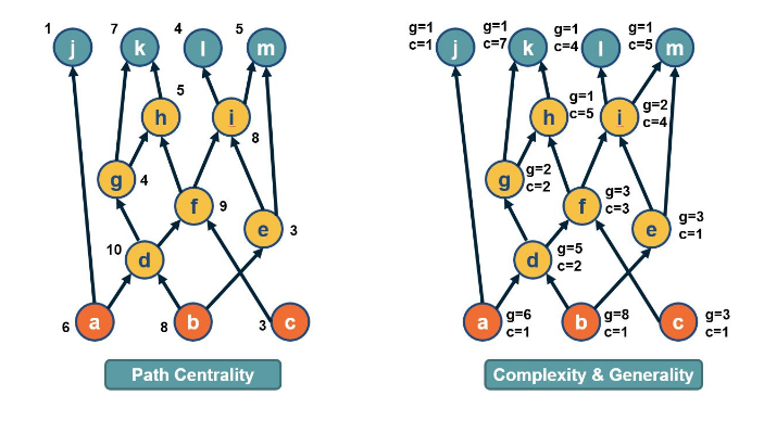
L6 Metric Summary¶

Degree (or strength) centrality: these metrics are more appropriate when we are interested in the number or weight of direct connections of each node. For example, suppose that you try to find the person with most friends in a social network.
Eigenvector/Katz/PageRank centrality: these metrics are more appropriate when we are mostly interested in the number of connections with other well-connected nodes. For example, suppose that you analyze a citation network and you try to identify research papers that are not just cited many times – but they are cited many times by other well-cited papers. For undirected networks, it is better to use Eigenvector centrality because it does not depend on any parameters. For directed networks, use Katz or PageRank depending on whether it makes sense to split the centrality of a node among its outgoing connections. For instance, this splitting may make sense in the case of Web pages but it may not make sense in the case of citation networks.
Closeness (or harmonic) centrality: these metrics are more appropriate when we are interested in how fast a node can reach every other node. For example, in an epidemic network, the person with the highest closeness centrality is expected to cause a larger outbreak than a person with very low closeness centrality. If the network includes multiple connected components, it is better to use harmonic centrality.
Betweenness centrality metrics: these metrics are more appropriate in problems that involve some form of transfer through a network, and the importance of a node relates to whether that node is in the route of such transfers. For example, consider a data communication network in which you want to identify the most central router. You should use a betweenness centrality that captures correctly the type of routes used in that network. For instance, if the network uses shortest-path routes, it makes sense to use shortest-path betweenness centrality. If however, the network uses equally all possible routes between each pair of nodes, the path centrality may be a more appropriate metric.

K-Core Decomposition¶

In some applications of network analysis, instead of trying to rank individual nodes in terms of centrality, we are interested in identifying the most important group of nodes in the network. There are different ways to think about the importance of groups of nodes. One of them is based on the notion of k-core.

Definition
A k-core (or “core of order-k”) is a maximal subset of nodes such that each node in that subset is connected to at least k others in that subset.

Note that, based on the previous definition, a node in the k-core also belongs to all lower cores, i.e., to any k'-core with k'< k.

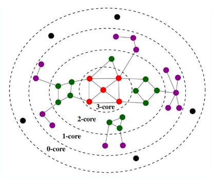
The visualization shows a network in which the red nodes belong to a core of order-3 (the highest order in this example), the green and red nodes form a core of order-2, while all nodes (except the black) form a core of order-1. Note that there is a purple node with degree=5 – but its highest order is 1 because all its connections except one are to nodes of degree-1. Similarly, there are green nodes of degree-3 that are in the 2-core set.

The nodes in the maximum core order are considered as the most well-connected group of nodes in the network.

Core-Periphery Structure

The nodes of such structures can be divided into two groups

a) Core Nodes: Which are very densely connected to each other and the rest of the network.
b) Periphery Nodes: Are well connected only to core nodes - not to other periphery networks

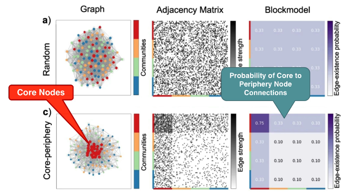
Rich-Club¶

A common approach for the detection of core-periphery structure is referred to as the rich-club of a network. The metaphor behind this concept comes from social networks: the very rich people are few and they have a large number of acquaintances, which include the rest of those few very rich people.

For general undirected networks

Let $n_k$ be the number of nodes with degree greater than k
Let $e_k$ be the edges between the $n_k$ nodes
- the nax number of edges will be $n_k(n_k - 1)/2$
Rich-Club Coefficient is given by
- $\large \phi(k) \frac{2 e_k }{n_k(n_k - 1)}$
- which quantifies the density of the connections between nodes of degree greater than k

This begs the question: How can we tell if $\phi(k)$ is statistically significant for a given k? Even random networks have about the same $\phi(k)$ for some degree values.

To test we generate an ensemble of random networks with the same number of nodes and degree distribution, just as we did for network motifs. If the rich-club coefficient for degree k in the given network is much larger than the corresponding coefficient in the null model, we can mark that value of k as statistically significant for the existence of a rich-club. If there is at least one such statistically significant value of k, we conclude that the network includes a rich-club -- the set of nodes with degree greater than k. If there are multiple such values of k, the rich-club nodes can be identified based on the value of k for which we have the largest difference between the rich-club coefficient in the real network versus the null model (even though there is some variation about this in the literature).

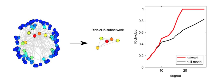
The visualization shows a synthetic network (left). The plot at the right shows the rich-club coefficient as a function of the degree k for the given network (red) as well as for the null model. The value of k for which we are most confident that a rich-club exists is k=19. There are five nodes with degree greater than 19 –they are shown (separately than the rest of the network) at the center of the visualization. Note that the corresponding rich-club coefficient is 1, which means that these five nodes form a clique. If we had chosen a higher value of k, the rich-club would only consist of a subset of these five nodes.

Tau-core set of Nodes for DAGs¶

A path-based approach to identify a group of core nodes in a network is referred to as the $\tau$-core”.

We define that a node v “covers” a path p when v is traversed by p.

The $\tau$-core is defined as follows:

given a set of network paths P we are interested in,
what is the minimal set of nodes that can cover at least a fraction $\tau$ of all paths in P?

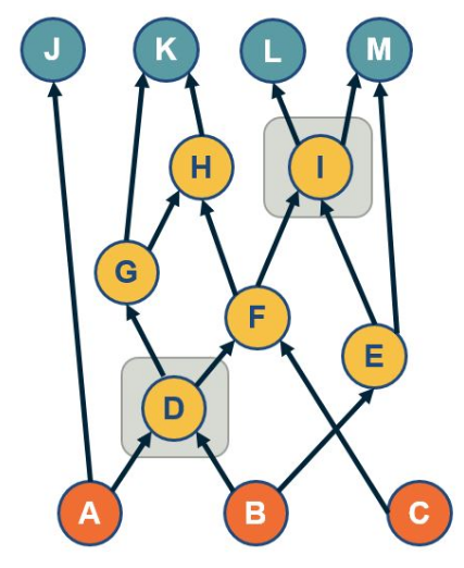
In the context of DAGs, the set P can be the ST-paths from the set of all sources (orange nodes) to all targets (blue nodes). The visualization shows the two core nodes (d and i) for the value of $\tau$=80%. Note that there are three ST-paths (a-j, b-e-m and c-f-h-k) that are not covered by this core set.

The rationale for covering only a fraction $\tau$ of paths (say 90%) instead of all paths is because in many real networks there are some ST-paths that do not traverse any intermediate nodes.

The problem of computing the the $\tau$-core has been shown to be NP-Complete It can be approximated by a greedy heuristic that iteratively selects the node with the maximum number of remaining un-covered paths until the constraint is met.

Examples

Game of Thrones: Here's a little analysis of the main characters from Game of throne using our centrality metrics

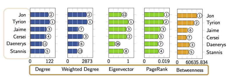
C.elgens $\tau$-core

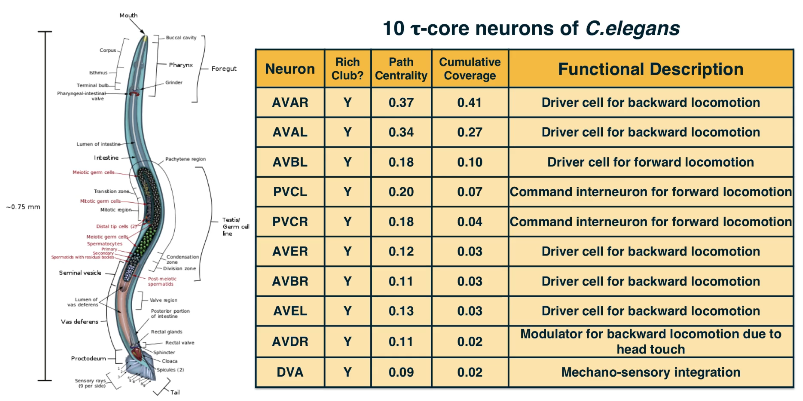
$\tau$

L7 Community Detection + Hierarchical Modularity¶

Objectives:

Understand the community detection problem
Utilize the modularity metric and appreciate its limitations
Analyze and deploy algorithms for community detection
Understand the notion of hierarchical modularity

Required Reading

Chapter-9 from A-L. Barabási, Network Science , 2015.
http://networksciencebook.com/chapter/9

Graph Partitioning¶

Minimum Bisection Problem
Given a graph, how do we partition the nodes into two non-overlapping sets of the same size s.t. we minimize the number of edges between the two sets? We are also general versions of this problem in which we partition the network into K non-overlapping sets of the same size, where K>2 is a given constant.

The graph partitioning problem is NP-Complete and so we only have efficient algorithms that can approximate its solution. The Kerninghan-Lin algorithm – as shown in the visualization below -- iteratively switches one pair of nodes between the two sets of the partition, selecting the pair that will cause the largest reduction in the number of edges that cut across the partition.

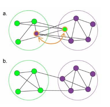
For our purposes, it is important to note that in the graph partitioning problem we are given the number of sets in the partition and that each set should have the same size. As we will see, this is very different than the community detection problem.

Community Detection¶

In the community detection problem, we also need to partition the nodes of a graph into a set of non overlapping clusters or communities. But the key difference is that we do not know a priori how many sets communities exist and there is no requirement that they have the same size.

What is the key property of its community?

Loosely speaking, the nodes within its community should form a densely connected sub-graph. This could mean a maximally sized clique, ie a complete sub graph that cannot be increased any further. This is a stringent definition however, and it does not capture the pragmatic fact that some edges between nodes of a community may be missing. So another way to think of its community is as an approximate clique, a sub graph in which the number of internal edges In other words, edges between nodes of the sub graph is much larger than the number of external edges, edges between nodes of that sub graph and the rest of the graph. This is again a rather loose definition, however, and it does not tell us which community is better the purple at the left or the green at the right.

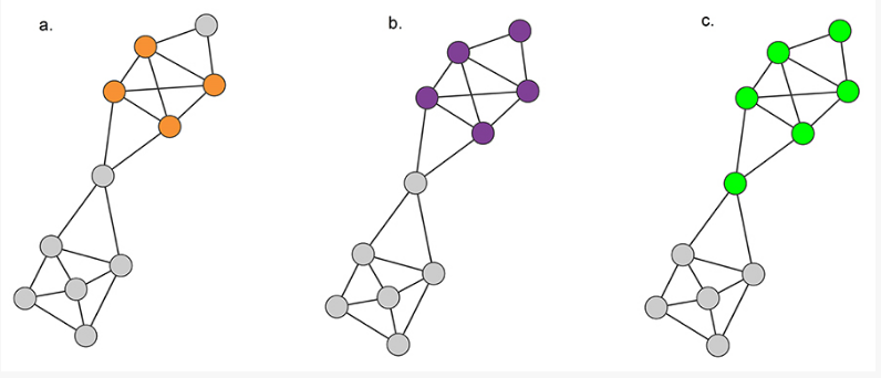
Some questions that may arise when trying to detect a community

Should every node belong to a community
Is it necassary that communities are non-overlapping?
- what if some nodes belong to more than one community?
What if there are no real communities in a network?
- What if the network is randomly formed?

Another way to think about network communities and visualize that presence is through the adjacency matrix. Suppose that there are k non-overlapping groups of nodes of potentially different sizes, so that the density of the internal connections within its group is much greater than the density of external connections. If we reorder the adjacency matrix of the network, so that the nodes of its group appear in consecutive rows, we will observe that the adjacency matrix includes k dense sub matrices one for each community.

The rest of the adjacency matrix is not completely zeros, but it is much more sparsely populated. This is shown in the visualization for a network with four communities, the red, the blue, the green, and the yellow.

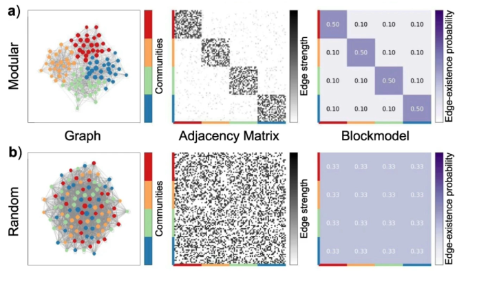
In this case, all four communities have the same size. The probability that two nodes of the same community are connected is 50%. The density of the external edges is only 10%.

CD using Centrality Metrics¶

A family of algorithms for community detection is based on hierarchical clustering. The goal of such approaches is to create a tree structure, or “dendrogram”, that shows how the nodes of the network can iteratively split in a top-down manner into smaller and smaller communities (“divisive hierarchical clustering”) – or how the nodes of the network can be iteratively merged in a bottom-up manner into larger and larger communities (“agglomerative hierarchical clustering”).

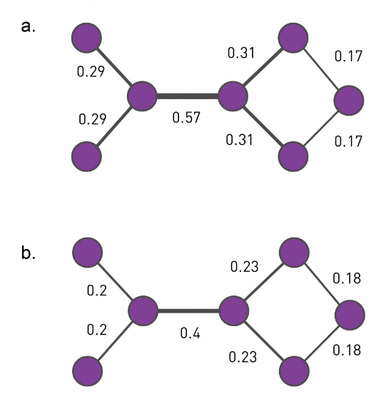
Let us start with divisive algorithms(visual above). We first need a metric to select edges that fall between communities – the iterative removal of such edges will gradually result in smaller and smaller communities.

One such metric is the edge (shortest path) betweenness centrality, introduced in Lesson-6. Recall that this metric is the fraction of shortest paths, across all pairs of terminal nodes, that traverses a given edge. Visualization (a) shows the value of the betweenness centrality for each edge. Removing the edge with the maximum centrality value (0.57) will partition the network into two communities. We can then recompute the betweenness centrality for each remaining edge, and repeat the process to identify the next smaller communities. This algorithm is referred to as "Girvan-Newman" in the literature.

Another edge centrality metric that can be used for the same purpose is the random walk betweenness centrality. Here, instead of following shortest paths from a node u to a node v, we compute the probability that a random walk that starts from u and terminates at v traverses each edge e, as shown in visualization (b). The edge with the highest such centrality is removed first.

Note that the computational complexity of such algorithms depends on the algorithm we use for the computation of the centrality metric. For betweenness centrality, that computation can be performed in O($LN$), where L is the number of edges and N is the number of nodes. Given that we remove one edge each time, and need to recompute the centrality of the remaining edges in each iteration, the computational complexity of the Girvan-Newman algorithm is O($L^2 N$). In sparse networks the number of edges is in the same order with the number of nodes, and so the Girvan-Newman algorithm runs in O($N^3$).

Girvan-Newman algorithm - Divisive¶

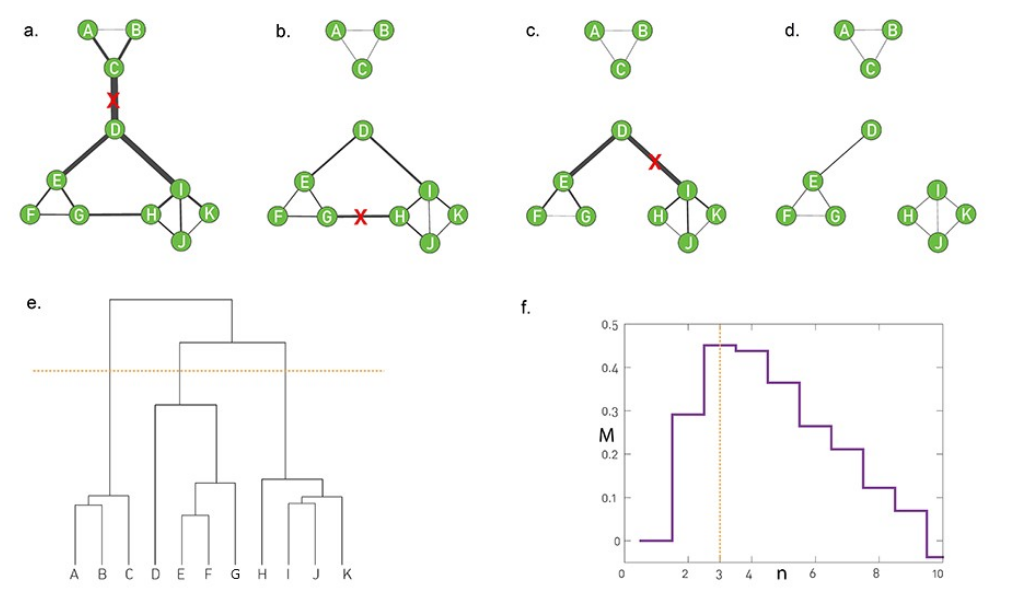
9.12 from networksciencebook.com The final steps of a divisive algorithm mirror those we used in agglomerative clustering:

Compute the centrality $x_ij$ of each link.
Remove the link with the largest centrality. In case of a tie, choose one link randomly.
Recalculate the centrality of each link for the altered network.
Repeat steps 2 and 3 until all links are removed.

The Girvan-Newman algorithm uses the betweenness centrality metric to remove a single edge in each iteration – the edge with the highest edge betweenness centrality. The value of the edge betweenness centrality of the remaining edges has to be re-computed because the set of shortest paths changes in each iteration.

The visualizations (a) through (d) show how a toy network changes in four steps of the algorithm, after removing three successive edges. The removal of the first edge, between C and D, creates the first split in the dendrogram, starting at the root. At the left, we have a community formed by A, B, and C – while at the right we have a community with all other nodes.

The next split takes place after we remove two edges, the edge between G and H and the edge between D and I. At that branching point the dendrogram shows three communities: (A,B,C), (D,E,F,G) and (H,I,J,K) (as shown by the horizontal yellow line).

The process can continue, removing one edge at a time, and moving down the dendrogram, until we end up with isolated nodes.

Note that a hierarchical clustering process does NOT tell us what is the best set of communities – each horizontal cut of the dendrogram corresponds to a different set of communities. So we clearly need an additional objective or criterion to select the best such set of communities. Such a metric, called modularity M, is shown in the visualization (f), which suggests we cut the dendrogram at the point of three communities (yellow line). We will discuss the metric M a bit later in this lesson.

This algorithm always detect communities in a given network. So, even a random network can be split in this hierarchical manner, even though the resulting communities may not have any statistical significance.

Agglomerative Hierarchical Clustering¶

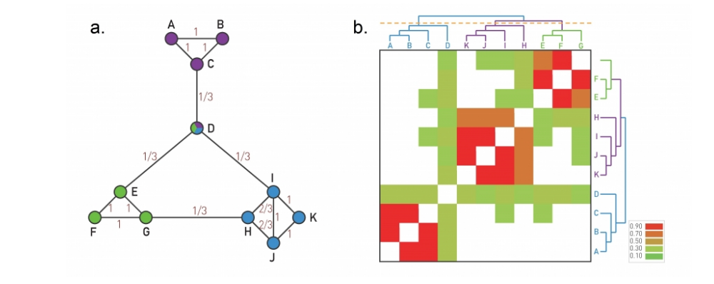
left shows the node similarity value for each pair of connected nodes
right shows the color-coded node similarity matrix, for every pair of nodes (even those not connected)

Here, we start the dendrogram at the leaves, one for each node. In each iteration, we decide which nodes to merge so that we extend the dendrogram by one branching point towards the top. The merged nodes should ideally belong to the same community. So we first need a metric that quantifies how likely it is that two nodes belong to the same community.

If two nodes, i and j, belong to the same community, we expect that they will both be connected to several other nodes of the same community. So, we expect that i and j have a large number of common neighbors, relative to their degree.

To formalize this intuition, we can define a similarity metric between any pair of nodes i and j:
$ \large S_{i,j} = \frac{ N_{i,j}+A_{i,j} }{min(k_i,k_j)} $
Where

$N_{i,j}$ is the number of common neighbours of i and j
$A_{i,j}$ is the adjacency matrix element for the two nodes
$k_i$ is the degree of node i

Observe that

$S_{i,j} = 1$
- if the two nodes are connected with each other
- and every neighbour of the lower-deg node is also a neighbour of the other node
$S_{i,j} = 0$
- when the nodes are not connected and they have no common neighbours

Group Similarity (Hierarchical)¶

There are three ways to do this:

Single linkage: the similarity of groups 1 and 2 is determined by the minimum distance (i.e., maximum similarity) across all pairs of nodes in groups 1 and 2.
Complete linkage: the similarity of groups 1 and 2 is determined by the maximum distance (i.e., minimum similarity) across all pairs of nodes in groups 1 and 2.
Average linkage: the similarity of groups 1 and 2 is determined by the average distance (i.e., average similarity) across all pairs of nodes in groups 1 and 2.

Now that we have defined a similarity metric for two nodes (based on the number of common neighbors), and we have also learned how to calculate a similarity value for two groups of nodes, we can design the following iterative algorithm to compute a hierarchical clustering dendrogram in a bottom-up manner. We start with each node represented as a leaf of the dendrogram. We also compute the matrix of $N^2$ pairwise node similarities.

In each step, we select the two nodes, or two groups of nodes more generally, that has the highest similarity value – and merge them into a new group of nodes. This new group forms a larger community and the corresponding merging operation corresponds to a new branching point in the dendrogram.

The process completes until all the nodes belong in the same group (root of the dendrogram).

Note that depending on where we “cut” the dendrogram we will end up with a different set of communities. For instance, the lowest horizontal yellow line at the visualization corresponds to four communities (green, purple, orange, and brown) – note that node D forms a community by itself.

The computational complexity of this algorithm, which is known as Ravasz algorithm, is O($N^2$) because the algorithm requires:

O($N^2$) for the initial calculation of the pairwise node similarities
O($N$) for updating the similarity between the newly formed group of nodes and all other groups – and this is performed in each iteration, resulting in O($N^2$)
O(N log N) for constructing the dendrogram

Modularity Metric¶

The unanswered questions from above is :

which partition of nodes into communities is best
are these communities statistically significant

Modularity metric is the answer to these problems. The idea is that randomly wired networks should not have communities -- and so a given community structure is statistically significant if the number of internal edges within the given communities is much larger than the number of internal edges if the network was randomly rewired (but preserving the degree of each node).

Formally
Suppose we're given a Network G(N,L), undirected and unweighted. Let $k_i$ be the degrees of the i'th node, and let C be a hypothetical partition into a set of communities $C_1,C_2,...,C_c$, let A be our Adjacency matrix.

The number of internal edges between all nodes of communicty $C_c$ is

$\large \frac{1}{2} \sum_{(i,j) \in C_c} A_{i,j}$

If the connections were made randomly then the expected number would be

$\large \frac{1}{2} \sum_{(i,j) \in C_i} \frac{k_i k_j}{2L}$
since node i has $k_i$ stubs and the probability that it connects to node-j is $\frac{k_j}{2L}$

We can take the delta as our modularity metric

$\large M = \frac{1}{2L} \sum_{c=1}^C \sum_{(i,j) \in C_c} ( A_{i,j} - \frac{k_i k_j}{2L} )$
we select the communities that have the largest modularity value

This can be further simplified to

$\large M = \sum_{c=1}^C (\frac{L_c}{L} - (\frac{k_c}{2L})^2 ) $
which expresses the modularity of a given community assignment as a summation, across all communities, of the following difference: the fraction of network edges that are internal to community $C_c$ MINUS the squared fraction of total edge stubs that belong to that community.

To test significance there are two approaches

a) Compare to network with M=0, which would be expected from a randomly wired network
b) compare to an ensemble of random networks, preserving degrees,
- then use a one-sided hypothesis test

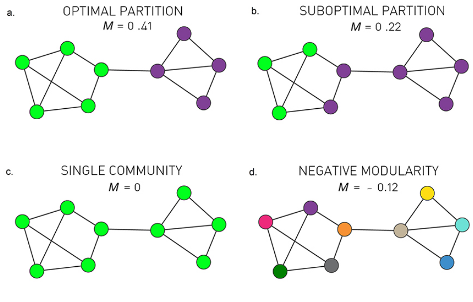
The visualization shows four possible community assignments.

The first two assignments have two communities. Assignment (a) is what we would expect visually and it has a modularity of M=0.41. It turns out that this is the highest possible modularity value for this network.
Assignment (b) is clearly a suboptimal community structure -- and indeed it has a lower modularity value (M=0.22)
Assignment (c) assigns all nodes to the same community – resulting in a modularity value of 0. Clearly this is not a statistically significant community.
Finally, assignment (d) assigns each node to its own community, resulting in a negative modularity value.

Now that we have a way to compare different community assignments, we can return to the hierarchical clustering approaches we saw earlier (both divisive and agglomerative) and add an extra step, after the construction of the dendrogram:

Each branching point of the dendrogram corresponds to a different community assignment, i.e., a different partition of the nodes in a set of communities. So, we can calculate the modularity at each branching point, and select the branching point that leads to the highest modularity value.

Unweighted and/or directed Networks

Modifiying the modularity metric

For Directed networks

$\large M = \frac{1}{L} \sum_{c=1}^C \sum_{(i,j) \in C_c} ( A_{i,j} - \frac{k_{i,out} k_{j,in}}{L} )$

For directed and weighted

$\large M = \frac{1}{S} \sum_{c=1}^C \sum_{(i,j) \in C_c} ( A_{i,j} - \frac{s_{i,out} s_{j,in}}{S} )$
where S is the sum of all weights

Modularity after merging¶

How does the modularity metric change upon the merging of two or more communities?

Suppose we have two communities A and B, with internal links $L_A$ and $L_B$, and total degrees $k_A$ and $k_B$. We wish to merge them into one community, while leaving all other communities the same?

first we observe that the number of links in the new community is $L_{AB} = L_A + L_B + l_{AB}$
- where $l_{AB}$ is the number of external links between A and B
2nd the total degree is $k_{AB} = k_{A} + k_{B}$
- straight forward
Now we can just use our formula from above/previous
$\large \Delta M_{AB} = (\frac{L_{AB}}{L} - (\frac{k_{AB}}{2L})^2 ) - ( \frac{L_A}{L} - (\frac{k_A}{2L})^2 + \frac{L_B}{L} - (\frac{k_B}{2L})^2 ) $
which can be simlified as
- $\large \Delta M_{AB} = \frac{l_{AB}}{L} - \frac{k_A k_B}{2L^2}$

This is a useful expression, showing that the merging step results in higher modularity only when the number of links between A and B is sufficiently large for the first term to be larger than the second term. And the larger the communities A and B are, the larger the second term is. Otherwise, this merging operation causes a reduction in the modularity of the new community assignment.

Modularity Maximization Greedy¶

Algo

Assign each node to a community, starting with N communities of single nodes
Inspect each community pair connected by at least 1 link and compute the modularity difference $\Delta M$ obtained if we merge those communities. Identify the community pair for which $\Delta M$ is the largest and merge them
- just use the formula from above
Repeat step 2 until all nodes merge into a single community - record the value of M at each iteration
- this effectively creates a dendogram in a bottom up manner
Select the iteration/partition for which M is maximal

Computational Complexity
Since the calculation of each ΔM can be done in constant time, Step-2 of the greedy algorithm requires O(L) computations. After deciding which communities to merge, the update of the matrix can be done in a worst-case time O(N). Since the algorithm requires N–1 community mergers, its complexity is O((L + N)N), or $O(N^2)$ on a sparse graph.

Optimized Greedy Algorithm
The use of data structures for sparse matrices can decrease the greedy algorithm’s computational complexity to O(N log2N). For more details please read the paper "Finding community structure in very large networks", by Clauset, Newman and Moore.

Modularity Maximization Louvain¶

First note that the Louvain algorithm will create a weighted network, even if passed an unweighted one.

Step 1

Assign each node to a different community
- for each node i evaluate the change in modularity when it is moved to the community of any of it's neighbours j
- Move i to the community for which the increase is the greatest.
- if it cannot be increased then leave it in it's original community
- repeat above steps until no improvement can be achieved

Step 2

We now construct a new network, weighted, whose nodes are the communities identified in Step 1
- The weight of the links between two nodes in this network is the sum of weights of all links between nodes in the corresponding two communities.
- Links between nodes of the same community lead to weighted self loops

Each pass consists of both of the above steps, Steps 1&2 are repeated in successive passes. The number of communities decreases in each pass, until there are no more changes. At this point maximum modularity is attained.

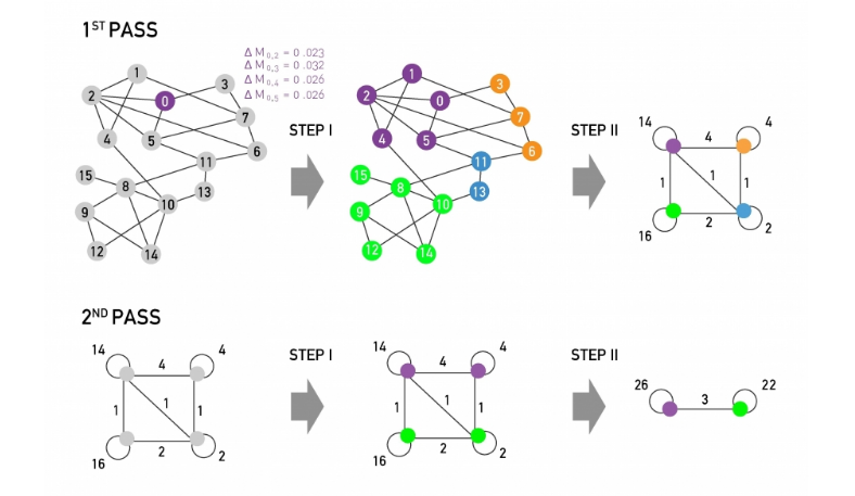
The visualization shows the expected modularity change $\Delta M_{0,i}$ for node 0. Accordingly, node 0 will join node 3, as the modularity change for this move is the largest, being $\Delta M_{0,3}=0.032$.

This process is repeated for each node, the node colors corresponding to the resulting communities, concluding Step-I.

In Step-II, the communities obtained in Step-I are aggregated, building a new network of communities. Nodes belonging to the same community are merged into a single node, as shown on the top right.

This process generates self-loops, corresponding to links between nodes in the same community that is now merged into a single node.

Modularity Resolution¶

Modularity Metric Shortcoming

Cannot be used to discover very small communities, small is relative to teh size of the network.

Recall our formula from earlier:

$\large \Delta M_{AB} = \frac{l_{AB}}{L} - \frac{k_A k_B}{2L^2}$

Suppose the total degree of each community is $k_l$. Then based on the formula the change after merging is

$\large \Delta M_{AB} = \frac{1}{L} - \frac{k_l^2}{2L^2}$
$=\frac{1}{L} ( 1 - \frac{k_l}{2L}^2)$

Merging will take place when $\Delta M_{AB} > 0$, this will occur when $k_l < \sqrt{2L}$. We can verbalize $\sqrt{2L}$ as the critical value. This scenario is called the Modularity Resolution because it is the smaller community size that a modularity maximization algorithm can detect. The consequence of all this is that a community with a degree less than the critical value will be merged, escaping detection.

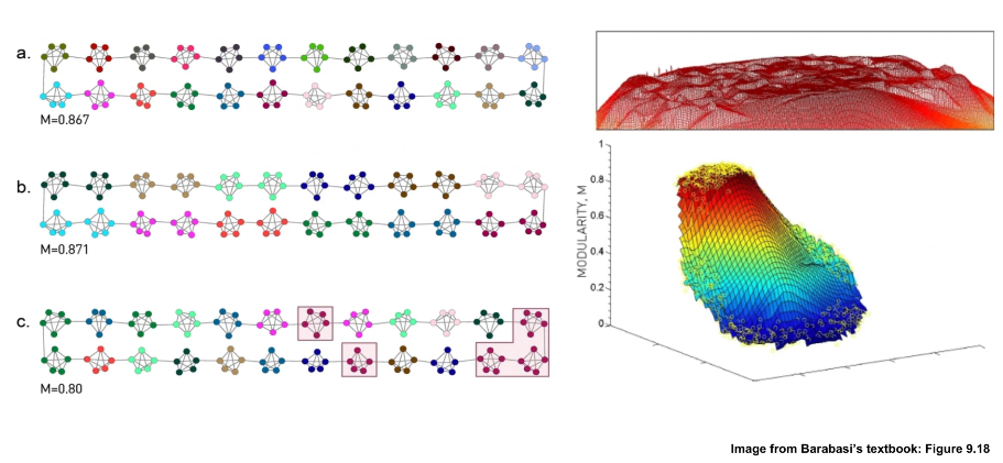
Consider the above illustration of a network. This is a ring network composed of Cliques. In the first stage we have a modularity metric of 0.867. Subsequent stages show possible configurations all with a higher modularity values. However, to get this some communities are merged into one, thereby losing their identity. In B we achieve the max modularity by grouping together every two.

This situation/event is actually quite common in practice. For starters computing the maximum modularity value is an NP-Hard problem. Secondly, the maximum modularity may not always correspond to the most intuitive sense of community. Notice the 3-dimensional image at right. There we can see the plateau's of various modularity values. So although we may not always be able to compute the maximum we can at least get to a pleateu where the values are quite close.

Communities within Communities¶

This describes a situation often found in real-world networks. For example consider a group of people working together on a project. They may only be one of many such groups in a larger project that in turn is embedded in a dept.

This is referred to as Hierarchical Modularity. Each module corresponds to a community of nodes. Smaller, more tightly connected communities can be members of larger but less tightly connected larger communities. This recursive process can continue for multiple levels until we reach a level in which the group of nodes is so loosely connected that they do not form a community anymore.

The nice thing about these networks is that they have a highly deterministic structure. The clustering coefficient of a node in this network drops proprotionally to the inverse of the node's degree: $C(k) \approx 2/k$. Furthermore, this acts like a call sign for such networks.

Clustering Coeff vs Degrees¶

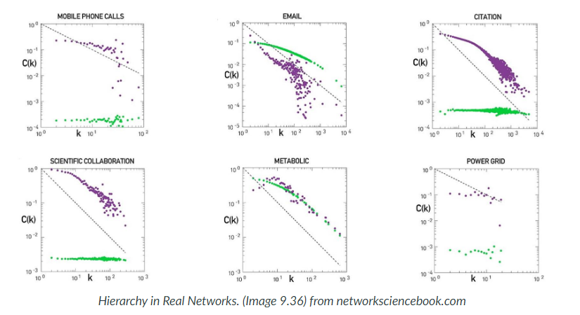
The visualization shows plots of the node clustering coefficient C(k) versus node degree k for six real-world networks (purple dots). You can find additional information about these six datasets in your textbook.

The green dots refer to a corresponding degree-preserving randomized network – this is an important step of the analysis because by randomizing the network connections (without changing the degree distribution), we remove the community structure of the original network from the randomized network.

The black dotted line corresponds to the relation C(k)=1/k. As we saw in the previous page, this is the slope of C(k) versus k in the deterministic hierarchically modular network that we saw earlier.

Note that some networks, such as the network of scientific collaborations or the citation network show clearly an inverse relation between C(k) and k, especially for nodes with degree k>10. Further, when we randomize the connections of those networks, removing the community structure, C(k) becomes independent of k. So, we expect that such networks exhibit a hierarchically modular structure.

Some other networks, such as the metabolic network or the email network, show an inverse relation between C(k) and k – but the same is true for the corresponding randomized networks! This raises the concern that the inverse relation between C(k) and k may be caused in some cases at least by the degree distribution – and not by the community structure of the network.

Finally, there are also networks in which we do not see a decreasing relation between C(k) and k, such as the mobile phone calls network or the power grid.

To summarize, hierarchical modularity is an important property of many (but not all) real-world networks, and when present, it exhibits itself with an inversely proportional between the clustering coefficient and the node degree. However, this relation is not sufficient evidence for the presence of hierarchical modularity.

Hierarchical Modularity Through Recursive Community Detection¶

Another approach to investigate the presence of hierarchical modularity is by applying a community detection algorithm in a recursive manner. The first set of discovered communities correspond to the top-level, larger communities. Then we can apply the same algorithm separately to each of those communities, asking whether there is a finer resolution community structure within each of those top-level communities. The process can continue until we reach a level at which a given community does not have a clear sub-community structure.

To illustrate this process, the visualization above refers to a collaboration network between about 55,000 physicists from all branches of physics who posted papers on arxiv.org. At the top-level (part a), the greedy modularity maximization algorithm detects about 600 communities and the modularity is M=0.713. The largest of those communities include about 13,500 scientists and 93% of them publish in condensed matter (C.M) physics. The second-largest community consists of about 11,000 scientists and 87% of those scientists publish in High Energy Physics (HEP).

If we apply the same community detection algorithm to the third-largest community, we identify a number of smaller communities, and the modularity of that community assignment is 0.807 (part b).

If we continue at a third level, applying the same algorithm to a community of 134 nodes we reach a point at which we identify research groups associated with scientists at different universities (part c).

L8 Advanced Community Detection¶

Learning Objectives

Identify overlapping communities
Generate synthetic networks with known community structure
Evaluate and compare community structures
Explain the role of nodes depending on their position between/within communities
Identify dynamic/evolving communities

Overlapping Nodes In practice, it is often the case that the network node may belong to more than one communities. Think of your social network. For instance, you probably belong to a community that covers mostly your family, another community of colleagues or classmates, a community of friends, and so on.

So how can we partition a network into non-overlapping communities, which you may recall was a fundamental assumption.

this is what we will discuss in the next few sections

CFinder¶

The cfinder algorithm was one of the first community detection algorithms that could detect overlapping communities. If k=3 cfinder looks for all triangles, Two k-cliques are considered overlapping if they share k-1 nodes. So for example two triangles are overlapping if they share a link.

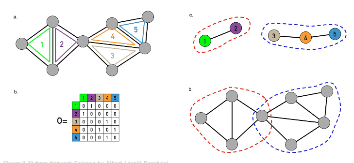
Consider the above illustration for k=3. In fig a we see the original network. In fig b we see the overlapping matrix O. Notice that there is a 1 to signal an overlapping between triangles. in fig (c) we see the connected components found by the CFinder algorithm, these are not the nodes. Finally fig (d) shows the original network with the connected components marked out. Now we can see the overlap experienced by the node at the centre.

Here is a more complex example

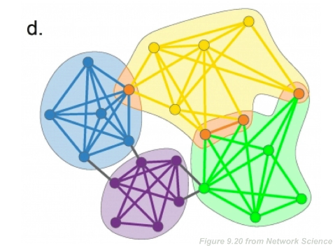
You might be wondering how the cfinder would work on a random G(N,p) network? If it is sufficiently dense then there is a good chance that for a low k communities will be found. After all there are bound to be small communities based purely on chance.

This begs the question: for what network size N and what k can we expect some communities by chance?
As it turns out the critical threshold is

$p_c(k) = [(k-1)n]^{-1/(k-1)}$
for a k-clique

For k=2, the k-cliques are simply individual links and the critical density threshold reduces to (1/n)

for k=3, the k-cliques become triangles and the critical density threshold is $p_c(k) = 1 / \sqrt{2n} $

A general rule of thumb when applying the Cfinder algorithm, we should also check whether the density of the network is below or above the critical threshold for the selected value of k. If it is larger than the threshold, we should consider larger values of k (even though this would make the algorithm more computationally intensive).

Link Clustering¶

This method is based on the idea that although a node may belong to multiple communities, a link should belong to only one. In a manner similar to the previous section, we will use the idea of clustering.

Similarity of nodes was done by looking for common neighbours,

So the similarity S( (i,k) , (j,k) ) of two links (i,k) and (j,k) that attach to a common node k can be evaluated based on the number of common neighbors that nodes i and j have – with the convention that the set of neighbors of a node i includes the node itself. We normalize this number by the total number of distinct neighbors of i and j, so that it is at most equal to 1 (when the two nodes i and j have exactly the same set of neighbors).

Let N(i) be the set of neighbours of i and let N(j) be the set of neighbours of j

then $\large S( (i,k) , (j,k) ) = \frac{ N(i)\cap N(j) }{N(i) \cup N(j)}$

Now that we have a similarity metric for pairs of links, we can follow exactly the same hierarchical clustering process we studied in the previous lesson to create a dendrogram of links, based on their pairwise similarity.

Cutting that dendrogram horizontally gives us different partitions of the set of network links – with each partition corresponding to a community assignment.

These communities, however, even though they are non-overlapping in terms of links, they may be overlapping in terms of nodes.

This is shown in the toy example of part-e: there are four clusters of links, corresponding to three communities of nodes. Note that two of the nodes belong to more than one community.

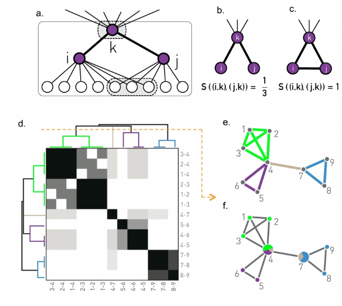
The computational complexity of the link clustering algorithm depends on two operations; 1) the similarity computation for every pair of links, and 2) the hierarchical clustering computation. The former depends on the maximum degree in the network, which we had derived earlier as O($n^{2/(\alpha -1)}$) [ in L4: Maximum Degree in a Power Law Network] for power-law networks with n nodes and degree exponent $\alpha$. The latter is O($m^2$), where m is the number of edges. For sparse networks, this last term is O($n^2$) and it dominates the former term.

GN Benchmark¶

Rhe gn benchmark is one of two algorithms for evaluating if an algorithm can detect communities. It is a synthetically generated network with a known community structure.

Girvan-Newman, aka GN, is the simplest of benchmarks. In this model all communities have the same size. Further any pair of nodes within a community have the same connection probability, $p_{int}$. Similarly any two nodes from different communities have the same connection probability, $p_{ext}$. Most importantly, because of these features the GN benchmark cannot be heavy-tailed.

let $n_c$ be the number of communities, and $N_c$ be the number of nodes in each community

then the total number of nodes is $N=n_c N_c$

Define

$\large \mu = \frac{k^{ext}}{k^{ext} + k^{int}}$
where $k^{int}$ is the avg number of internal connections in a community
and $k^{ext}$ is the avg number of external connections between communities

observe

When $\mu \rightarrow 0$ almost all connections are internal and the communities are clearly seperated
as $\mu$ increases the community structure weakens.
- At about $\mu=0.5$ we begin to see more external connections than internal

GN network with 128 nodes, four communities, and 32 nodes per community when $\mu$ is 40%.

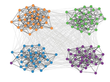
The GN benchmark creates communities of identical size. How realistic is this assumption, however?

Even though we typically do not have the ground-truth, there is increasing evidence that most networks have a power-law community size distribution. This implies that most communities are quite small, maybe a tiny percentage of all nodes, but there are also few large communities with comparable size to the whole network.

LFR Benchmark¶

LFR benchmark (Lancichinetti-Fortunato-Radicchi) is more realistic because it generates networks with scale-free degree distribution – and additionally, the community size follows a power-law size distribution.

We need to specify the total number of nodes n, the parameter $\mu$ that we also saw in the GN benchmark, two exponent parameters: $\gamma$ for the node degree distribution and $\zeta$ for the community size distribution, as well as the minimum and maximum values for the degree distribution and the community size distribution.

LFR starts with n disconnected nodes, giving each of them a degree (number of stubs) based on the degree distribution.

Also, each node is assigned to a community based on the community size distribution (see part-a and part-b).

The stubs of each node are then classified as either internal, to be connected to other internal stubs of nodes in the same community – or external, to be connected to available external stubs of nodes in other communities (see part-c). This stub partitioning process is controlled by the parameter of the GN benchmark.

The connections between nodes are then assigned randomly as long as a node has available stubs of the appropriate type (internal vs external) (see part-d).

The visualization part-e shows an LFR network with n=500, $\mu$=0.4, $\gamma$=2.5, and $\zeta$=2. Note that the 16 communities have very different sizes, and the nodes are also highly heterogeneous in terms of degree.

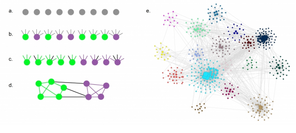
Normalized Mutual Information NMI metric¶

Suppose we have two community partitions P1 and P2, in the same network. We don't know how these partitions were determined nor how they measure up to the ground truth. So how can we compare these ?

To do this we need the joint distribution $p(C_i^1,C_j^1)$=Pr(node belongs to C_i of P1 AND node belongs to C_j of P2 )
Then we can determine the marginal probabilities: $p(C_i^1)$ and $p(C_j^1)$

Thankfully this can all be done by constructing a confusion matrix as shown below.

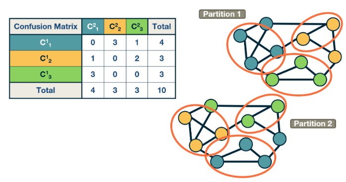
A common way to compare two statistical distributions in Information Theory is through the Mutual Information – this metric quantifies how much information we get for one of two random variables if we know the value of the other. If the two random variables are statistically independent, we do not get any information. If the two random variables are identical, we get the maximum information.

The normalized Mutual metric (NMI) is defined as

$\large NMI = I_n = \frac{\sum_{i,j} p(C_i^1,C_j^1) \log_2 \frac{p(C_i^1,C_j^1)}{p(C_i^1)p(C_j^1)} }{\frac{1}{2} [H(p(C^1)) + H(p(C^2))]}$

Notes:

the top term is the Mutual Information (unnormalized of course)
the bottom term is the average entropy of the two partitions,
- Entropy of a R.V. definition : $H(X) = -\sum_x p(x) \log_2 p(x) \log_2 p(x)$

Consider

What is minimum value of the mutual information metric results when the two partitions are statistically independent?
The maximum value results when they are identical.
Also, what is that maximum value?.

Algo Comparisons¶

Accuracy

In previous lessons, we covered the Girvan-Newman algorithm (top-down hierarchical clustering based on the edge betweenness centrality metric), the Ravasz algorithm (agglomerative hierarchical clustering), the greedy modularity optimization algorithm, and the Louvain algorithm (also based on modularity optimization). The plots also show results for Infomap, which is an algorithm that is based on the maximization of an information-theoretic metric of community structure rather than modularity.

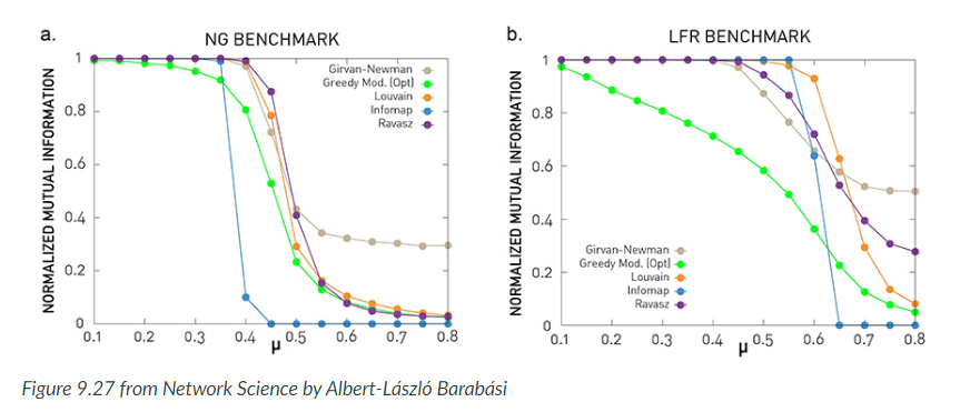
The comparisons use the NMI metric, and the two benchmarks we introduced earlier: GN and LFR. Recall that the parameter $\mu$ quantifies the strength of the community structure in the network – when $\mu$ < 0.5 the network has clearly separated communities, while $\mu$ is close to 1 there is no real community structure.

The benchmark parameters are N=1,000 nodes, average degree: $\bar{k}$=20, degree exponent (LFR) $\gamma$=2, maximum degree (LFR): $k_{max}$=50, community size exponent (LFR) $\zeta$=1, maximum community size (LFR): 100, minimum community size (LFR): 20. Each curve is averaged over 25 independent realizations.

Runtime

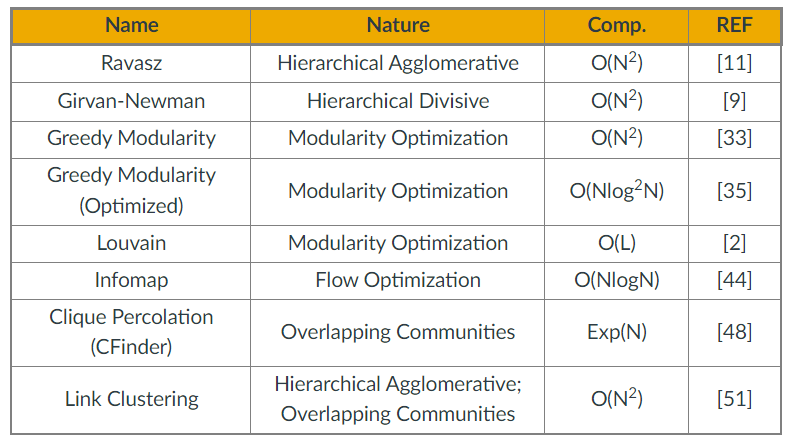
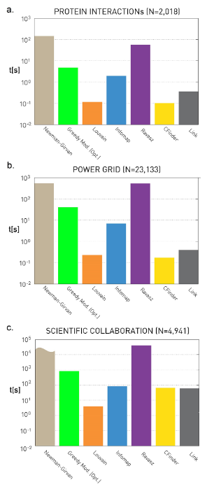
In sparse networks (where the number of links is L=O(N)) the Louvain algorithm is the fastest in terms of algorithmic complexity. In dense networks (where L=O(N^2)), the Infomap and greedy modularity maximization algorithms are faster.

These plots quantify the empirical run-time of the previous community detection algorithms for three small/medium network datasets. The y-axis values are in seconds.

As expected, the fastest algorithm is Louvain. Surprisingly, even though the Cfinder algorithm has an exponential worst-case run-time, it performs quite competitively in practice. The Newman-Girvan algorithm is the slowest among the seven algorithms.

Dynamic Communities¶

In practice, many networks change over time through the creation or removal of nodes and edges. This dynamic behavior also causes changes in the community structure of the network.

There are various ways in which the community structure may change from time t to time t+1

Growth: a community can grow through new nodes.
Contraction: a community can contract through node removals.
Merging: two or more communities can merge into a single community.
Splitting: one community can split into two or more communities.
Birth: a new community can appear at a given time.
Death: a community can disappear at any time.
Resurgence: a community can only disappear for a period and come back later.

The problem of detecting communities in dynamic networks is more recent and there is not a single method yet that is considered generally accepted. Most approaches in the literature follow one of the following three general approaches.

DC: Approach 1

The first approach is that a community detection algorithm is applied independently on each network snapshot, without any constraints imposed by earlier or later network snapshots.

Communities identified at time T+1 are matched to the communities identified at time T based on maximum node and edge similarity.
Some communities experience gradual growth while others may experiences contraction.

The main advantage of this approach is its simplicity, given that we can apply any algorithm for community detection on static networks.

Its main disadvantage however is that the communities of successive snapshots can be significantly different, not because there is a genuine change in the community structure, but because the static community detection algorithm may be unstable, producing very different results even with minor changes in the topology of the input graph.

DC: Approach 2

The second approach attempts to compute a good community structure at time T+1 also considering the community structure computed earlier at time T.

To do so, we need to modify the objective function of the community detection optimization problem: instead of trying to maximize modularity at time T+1, we aim to meet two goals simultaneously:
- have both high modularity at time T+1
- and maintain the community structure of time T as much as possible.
This is a trade-off between the quality of the discovered communities (quantified with the modularity metric) and the ”smoothness” of the community evolution over time.

Such dual objectives require additional optimization parameters and trade-offs, raising concerns about the robustness of the results.

DC: Approach 3

A third approach is to consider all network snapshots simultaneously. Or, a more pragmatic approach would be to consider an entire “window” of network snapshots (T,T+1,T+2,...,T+W-1) at the same time.

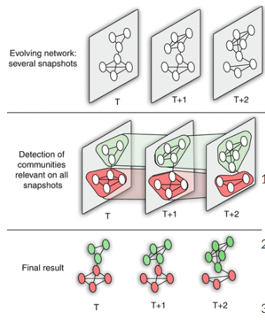
Algorithms of this type create a single “global network" based on all these snapshots as follows:

A node of even a single snapshot is also a node of the global network, and an edge of even a single snapshot is also an edge between the corresponding two nodes at the global network.
Additionally, the global network includes edges between the instances of any node X at different snapshots (so if X appears at time T and at time T+1, there will be an edge between the corresponding two node instances in the global network).
After creating the global network, a community detection algorithm is applied on that network to compute a “reference” community structure.
Then, that reference community structure is mapped back to each snapshot, based on the nodes and edges that are present at that snapshot.

This approach usually produces the smoothest (or most stable) results – but it can miss major steps in the evolution of the community structure (such as communities that merge or split). This last point however also depends on the length of the window W.

Participation Coefficient¶

Is a node a link/bridge between communities or is it mostly connected to other nodes in the same community. This is the question the participation coefficient trys to answer

Suppose we know that a Network has $n_c$ communities, and let $k_{i,s}$ be the number of links of node i that are connected to nodes of community s, and $k_i$ is the degree of node i
Then

$P_i = 1 - \sum_{s=1}^{n_c} (\frac{k_{i,s}}{k_i})^2 $

Observe:

when all connections of i are within the same community
- $P_i$ will be 0
when the connections of i are uniformly distributed among the communities
- $P_i$ will be close to 1
$P_i=1$ serves as an upper bound, it will be approached for nodes with a very large degree $k_i$ whose links are uniformly distributed

Within-module Degree¶

Normalized module degree:

$\large z_i = \frac{k_i - \bar{k}_i }{ \sigma_{k_i} }$
where
- $k_i$ is the internal degree of node i, within the same community
- $\bar{k}_i$ is the avg internal degree of all nodes in the same community
- $\sigma_{k_i}$ is the standard deviation of the internal nodes

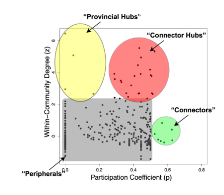
If we combine the information provided by both the participation coefficient and the within-community degree, as shown in the visualization, we can identify four types of nodes, based on the nodes that have unusually high values of $P_i$ and $z_i$:

Connector Hubs: nodes with high values of both $P_i$ and $z_i$. These are hubs within their own community that are also highly connected to other communities, forming bridges to those communities.
Provincial Hubs: nodes with high value of $z_i$, but low value of $P_i$. These are hubs within their own community but not well connected to nodes of other communities.
Connectors: nodes with high value of $P_i$, but low value of $z_i$. These are not hubs within their module – but they form bridges to other communities.
Peripheral nodes: nodes with low values of both $P_i$ and $z_i$. Everything else -- this is how the bulk of the nodes will be classified as.

Clearly, these four types are heuristically defined and there are always nodes that would fall somewhere between these four roles.

Delta Maps¶

Used primarily for spatial and temporal data. Such as that used in Climate patterns over time spanning a large geographic area.

Another use case is neural activity over time, like a series of MRI images. Here the activity time series may be EEG signals from different electrodes or FMRI measurements at different voxels. After delta maps detects the homogeneous communities or domains, it forms a weighted network between domains based on the strength of the statistical correlation between the aggregate signal of each domain pair.

Simplified presentation of the delta-MAPS method
For the full paper: https://link.springer.com/article/10.1007/s41109-018-0078-z

The input is a timeseries $x_i(t)$ for each grid point i. The similarity between two grid points i and j is quantified using Pearson's cross-correlation $r_{i,j}$. More advanced correlation metrics could be used instead (such as mutual information). Additionally, the correlation could be calculated at different lags. Links to an external site.

A domain A(s) with seed s (a specific grid point) is the largest possible spatially contiguous set of points including s such that their average pairwise correlation $\hat{r}(A)$ is greater than the parameter of the method $\delta$.

The objective of Delta-MAPS is to identify the minimum number of such maximal “domains” in the given data.

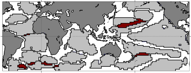
For example, the visualization shows the detected domains when Delta-MAPS is applied to Sea Surface Temperature (SST) monthly data (HadISST) for the time period of about 50 years (after removing the effects of seasonality). Each spatially contiguous region is a domain. You can think of a domain as a network community in which the nodes are grid points in space, and the edge weight between two nodes is equal to the cross-correlation of their activity time series.

Note that there are 18 such domains in this data. The red regions correspond to spatial overlaps between adjacent domains – Delta-MAPS allows for overlapping communities.

Another feature of the method is that not every node needs to belong to a community – as we see there are many grid points on the oceanic surface that do not belong to any domain.

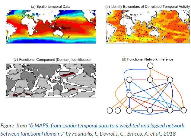
Here is a short overview of the Delta-MAPS algorithm:

The algorithm starts with a time series for each point in space (part-a shows the average of that time series for each grid point).

Then, Delta-MAPS selects potential domain seeds. These points are local maxima of the spatial correlation field (part-b, “epicenters of correlated temporal activity”).

Then, the algorithm proceeds iteratively, identifying one domain at a time. The domain identification starts by selecting the next available seed of maximum spatial correlation. The algorithm then selects, in a greedy manner, as many points as possible around the chosen seed so that it forms a maximal spatially contiguous block of points that satisfy the homogeneity constraint $\delta$ (part-c, “domain identification”).

Finally, the algorithm identifies functional connections between domains, based on how strong their pairwise correlations are. These correlations can be positive (red) or negative (blue), and lagged (part-d, “functional network inference”).

L9 Network Contagion and Epidemics¶

Learning Objectives

Define what “network contagion” means
Analyze standard network epidemic models in the context of realistic network models
Explain how the structure of a network can have a major effect on the function and dynamic activity on that network
Understand the role of superspreaders in epidemics

Common Modeling Strategies¶

First, the compartmental model,
- here the models assume that individuals belong to a small number of compartments such as susceptible, exposed, infected, or removed recovered.
- Such models do not capture the network structure of the population, instead, they assume that all individuals have the same number of contacts. The only difference between individuals is their epidemiological state, their compartment.
second one: is the vector-borne compartmental model.
- Here we consider both the vectors for example, the mosquitoes and the hosts, the humans have an infectious disease and their epidemiological state.
third class: the special models
- we also consider the population density at different locations.
- This is necessary when the goal of the model is to predict how an epidemic will spread in a country or city.
In the fourth class, the metapopulation models,
- here the population is modeled with two or more subpopulations.
- It's with different mobility, location, or transmission characteristics.
the fifth one,
- is network models, here we mostly focus on the network of contacts between individuals.
- The properties of this network, for example, that degree distribution can have major implications on the spread of an epidemic.
finally, individual based models
- are the most detailed, but also the most computationally intensive.
- Because here we have to capture what happens to each individual as he or she moves around.

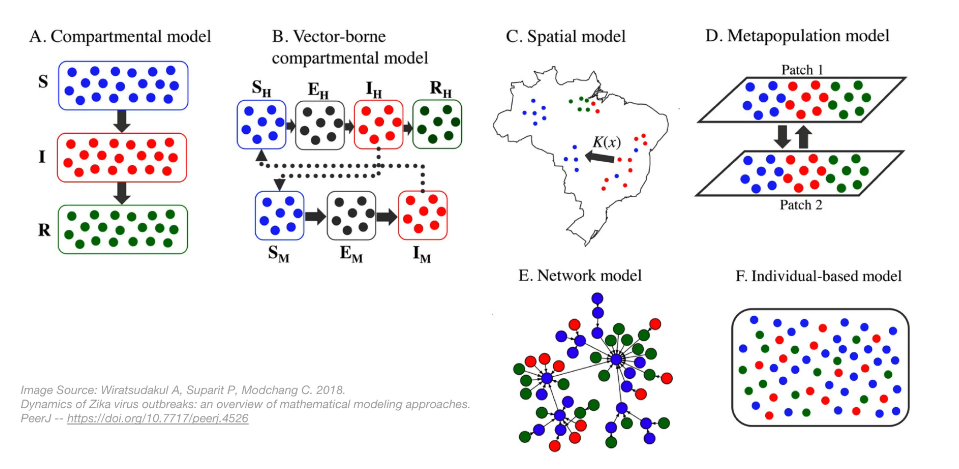
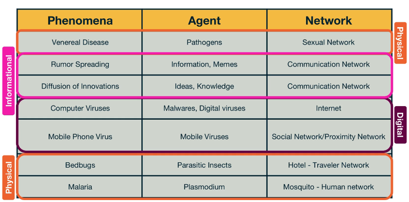
SI Model¶

In the SI model, there are two compartments: Susceptible (S) and Infected (I) individuals. To become infected, a susceptible individual must come in contact with an infected individual. If someone gets infected, they stay infected.

If S(t) and I(t) are the number of susceptible and infected individuals as functions of time, respectively, we have that S(t) + I(t) = N. We typically normalize these functions by the population size, and we work with the two population densities

$s(t) = S(t) / N$
$i(t) = I(t) / N$
where $s(t) + i(t) = 1$

Infection begins at time t=0
with a single infected individual $i(0) = 1/N = i_0$

Suppose that an S individual is in contact with only one infected individual. Let us define the parameter $\beta$ as follows: $\beta dt$ is the probability that S will become infected during an infinitesimal time interval of length $dt$.

Given that the S individual is in contact with $\bar{k}$ infected individuals, this probability increases to $1-(1-\beta dt)^{\bar{k}} \approx 1-(1-\bar{k} \beta dt)=\bar{k} \beta dt $ because the infection can take place independently through any of the infected contacts (the approximation is good as long as this probability is very small).

If the density of infected individuals is i(t), then the probability that the S individual becomes infected is $\bar{k} \beta i(t) dt$.

The infection process is always probabilistic but for simplicity, we can model it deterministically with a two-state continuous-time Markov process: an individual moves from the S to the I state with a transition rate $\beta i(t)$.

I'm going to leave out the gory details of the derivation, in a nutshell

The density of S individuals is s(t), the increase in the density of infected individuals during dt is:
- $di(t) = \bar{k} \beta i(t) s(t) dt$
yada yada
this is a nonlinear differential equation
the final closed-form solution for the density of infected individuals for $t \ge 0$
- $\large i(t) = \frac{i_0 e^{\bar{k}\beta t}}{(1-i_0) + i_0 e^{\bar{k}\beta t}}$

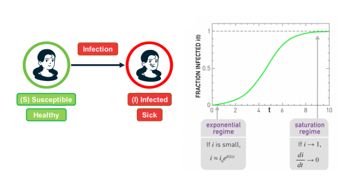
There are some important things to note about this function:

For small values of t, when the density of infected individuals is very small and the outbreak is only at its start, i(t) increases exponentially fast: $ i(t) \approx i_0 e^{\bar{k}\beta t}$
The time constant during that “exponential regime” is $\frac{1}{\bar{k} \beta}$. This time constant is often used to quantify how fast an outbreak spreads. This time constant decreases with both the infectiousness of the pathogen (quantified by $beta$) and the number of contacts $\bar{k}$.
For large values of t, the density of infected individuals tends asymptotically to 1 – meaning that everyone gets infected.

SIS Model¶

The SI model is unrealistic because it assumes that an infected individual stays infected. In practice, thanks to our immune system, we can recover from most infections after some time period. In the SIS model, we extend the SI model with an additional transition, from the I back to the S state to capture this recovery process.

The recovery of an infected individual is also a probabilistic process. As we did with the infection process, let us define as $\mu dt$ the probability that an infected individual recovers during an infinitesimal time period $dt$. If the density of infected individuals is i(t), then the transition rate from the I state to the S state is $\mu i(t)$.

SIS model can lead to two very different outcomes, depending on the magnitude of the recovery rate $\mu$ relative to the cumulative infection rate $\bar{k} \beta$:

when $\bar{k} \beta < \mu $
- then the exponent in the previous solution is negative and the density of infected individuals drops exponentially fast from $i_0$ to zero. In other words, the original infection does not cause an outbreak. This happens when the recovery of the original infected individual takes place faster than the infection of his/her susceptible neighbors.
when $\bar{k} \beta > \mu $
- we have an exponential outbreak for small values of t (when the density of infected individuals is quite smaller than 1). In that regime, we can approximate the solution of the SIS model with the following equation:
- $\large i(t) \approx i_0 e^{(\bar{k} \beta - \mu) t } $

the ratio $\frac{\bar{k} \beta}{\mu}$ is critical for the SIS model. If it is larger than 1, the SIS model predicts that even a small outbreak will lead to an endemic state. Otherwise, the outbreak will die out. This is why we define that the epidemic threshold of this model is equal to one.

SIR Model¶

For some pathogens (e.g., the virus VZV that causes chickenpox), if an individual recovers he/she develops persistent immunity (through the creation of antibodies for that pathogen) and so the individual cannot get infected again.

For other pathogens, such as HIV, there is no natural recovery and an infected individual may die after some time.

To model both possibilities, the SIR model extends the SI model with a third state R referred to as “Removed”. The transition from I to R represents that either the infected individual acquired natural immunity or that he/she died. In either case, that individual cannot infect anyone else and cannot get infected again.

As in the case of the SIS model, we will denote as $\mu$ the parameter that describes how fast an infected individual moves out of the infected state (independent of whether this transition represents recovery/immunity or death).

There are now three population densities, one for each state, and they should always add up to one:

$s(t) + i(t) + r(t) = 1$

Comparison of SI, SIS, SIR Models Under Homogeneous Mixing¶

Homogenous Mixing
The homogenous mixing hypothesis (also called fully mixed or mass-action approximation) assumes that each individual has the same chance of coming into contact with an infected individual. This hypothesis eliminates the need to know the precise contact network on which the disease spreads, replacing it with the assumption that anyone can infect anyone else.

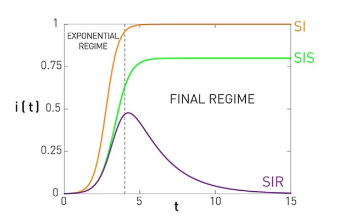
This figure summarizes the results for the SI, SIS, and SIR models, under the assumption of homogeneous mixing.

For the SI model there is no epidemic threshold and we always get an epidemic that infects the entire population.

For the SIS and SIR models we get an epidemic if the ratio $\frac{\bar{k}\beta}{\mu}$ is greater than the epidemic threshold, which is equal to one. In that case, both models predict an initial "exponential regime". The difference between the SIS and SIR models is that the former leads to an endemic state in which a fraction $1 - \frac{\mu}{\bar{k}\beta}$ of the population remains infected (if the epidemic threshold is exceeded).

There are more realistic models in the epidemiology literature, with additional compartmental states and parameters. A common such extension is to introduce an “Exposed” state E, between the S and I states, which models that individuals that are exposed to a pathogen stay dormant for some time period (until they develop enough viral load) before they become infectious. This leads to the SEIR model.

Another extension is to consider pathogens in which some infected individuals may acquire natural immunity while others may die. This requires to have two different Removed states, with different transition rates.

L9 Case Studies¶

Number of Partners in Sexual Networks¶

All previous derivations assume that each individual has the same number of contacts . This assumption makes the derivations simpler – but as we will see later in this lesson, it can also be misleading especially when the number of contacts of different individuals varies considerably.

Let us start with sexually transmitted diseases. The plot at the left shows the distribution of the number of sexual partners, separately for men and women, since sexual initiation in a 1996 survey in Sweden. Note that the plot is in log-log scale. The straight-line decay when the number of partners is larger than 20 suggests that the corresponding distribution follows a power-law. The exponent is about 3 for women and 2.6 for men. Even though most men had less than 10-20 partners, there are also individuals with 100s of partners.

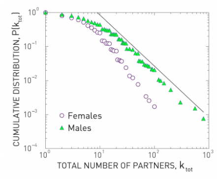
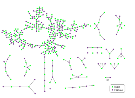
The plot at the right shows is based on a survey of high school students and “romantic relationships”. Note that even though there are 63 couples without any other connections and many other nodes with only 1-2 connections, there are also few nodes with a much higher number of such relationships (up to almost 10).

Assuming that every individual has the same number of contacts/partners would be very far from the truth at least in these two datasets. So, clearly, the homogeneous mixing assumption is very unrealistic.

Number of “Close Proximity” Contacts¶

For airborne pathogens and respiratory diseases such as COVID-19, what matters more is the number of individuals we are in close proximity to. This cannot be measured with surveys but it can be measured with wireless technology such as RFID badges (Radio Frequency Identification) . Various studies have provided volunteers with RFID badges and asked them to wear them throughout the whole day (e.g., on university campuses, dorms, gyms) .

A common conclusion from these studies is that the number of people we come close to varies greatly across individuals. Most of us come physically close to only a small number of specific other people but some individuals interact with hundreds of other people in their daily life. RFID technology can also give us information about the duration of these interactions, which is also a very important factor in the transmission of a pathogen from an infected to a susceptible individual.

The statistical distribution of these durations is also heavy-tailed, typically following a power-law, meaning that most of our face-to-face interactions are very brief (e.g., saying hi at a corridor) but few interactions last for hours – and typically those are the most dangerous for the transmissions of viruses such as COVID-19, H1N1, influenza, etc.

Global Travel Network¶

Another important factor in the spread of pathogens is the global travel network. Especially with air transportation, in the last few decades, it has become possible for an airborne virus to spread from one point of the planet to all major cities around the world within the first 24 hours.

Imagine, for instance, an infected individual sneezing while waiting at the security control line of a busy airport such as JFK. The passengers around him/her may be traveling to almost every other country on the planet.

R0 Reproductive Number¶

R0, is roughly defined as: the average number of secondary infections that arise from a single infected individual in a susceptible population.

One way to estimate R0 is to multiply the average number of contacts of an infected individual by the probability that a susceptive individual will become infected by a single infected individual (“attack rate AR”). So, the R0 metric does not depend only on the given pathogen – it also depends on the number of contacts each individual has.

If the number of secondary infections from a single infected individual is R0>1 then an outbreak is likely to become an epidemic, while if R0<1 then an outbreak will not spread beyond a few initially infected individuals.

In the context of SIS & SIR models we can show that $R_0 = \bar{k} \beta / \mu $

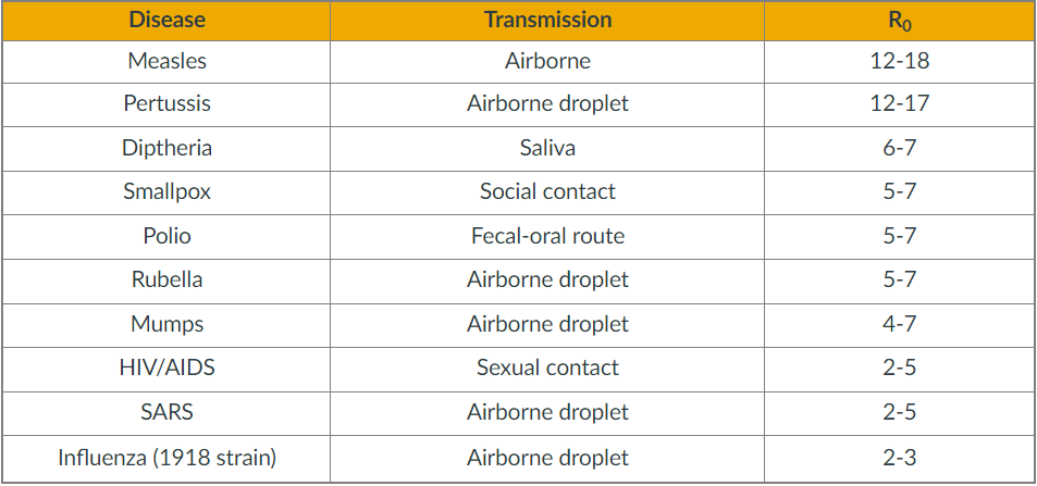
R0 is only an average

it does not capture the heterogeneity in the number of contacts of different individuals (and it also does not capture the heterogeneity in the “attack rate” or “shedding potential” of the pathogen at different individuals). As we know by now, contact networks can be extremely heterogeneous in terms of the degree distribution, and they can be modeled with a power-law distribution of (theoretically) infinite variance. Such networks include hubs – and hubs can act as "superspreaders" during outbreaks.

It is important to note the presence of a few hub nodes, referred to as superspreaders in the context of epidemics. The presence of superspreaders emphasizes the role of degree heterogeneity in network phenomena such as epidemics. If the infection network was more “Poisson-like”, it would not have superspreaders and the total number of infected individuals would be considerably smaller.

”Superspreading events” (SSE) are events during an outbreak in which a single infected individual causes a large number of direct or indirect infections. SSEs have been observed in practically every epidemic – and they have major consequences both in terms of the speed through which an epidemic spreads and in terms of appropriate interventions.

For example, in the case of respiratory infections (such as COVID-19) “social distancing” is an effective intervention only as long as it is adopted widely enough to also include superspreaders.

To avoid the homogeneous mixing assumption, one option would be to model explicitly the state (e.g., susceptible, infected, removed) of each node in the network, considering the degree of that node. That would result in a large system of differential equations that would only be solvable numerically.

Another approach is to group all nodes with a certain degree k together in the same “block”. Then, we can ask questions such as: what is the rate at which nodes of degree k move from the S to the I state? In other words, we will not be able to make specific predictions for individual nodes but will be able to characterize the compartmental dynamics of all nodes that have a certain degree. This is referred to as the “degree block approximation.”

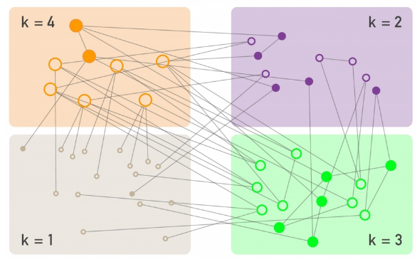
SIS - degree block approximation¶

SIS Model differential equation becomes

$\large \frac{di_k(t)}{dt} = k \beta \theta_k(t) (1 - i_k(t)) - \mu i_k(t) $
which after a lot of math solves to
- $\large ce^{t(\beta \bar{k}^2 - (\beta + \mu)\bar{k})/\bar{k}}$

This says that there will be an outbreak IFF $ (\beta \bar{k}^2 - (\beta + \mu)\bar{k}) > 0 $
Whereas under homogenous mixing this was $ (\beta \bar{k} - \mu) > 0 $

In other words, when we consider an arbitrary degree distribution, it is not just the average degree that affects the epidemic threshold. The second moment of the degree distribution also matters. And as the second moment increases relative to the first (i.e., the ratio $\bar{k} / \bar{k}^2$ decreases), it is easier to get an epidemic outbreak.

SIS Model – No Epidemic Threshold For Scale-Free Nets

Recall that in a random network with a Poisson degree distribution (Like ER Networks)

Variance == mean
and the second moment is $\bar{k}^2 = \bar{k}(1 - \bar{k})$

Thus we get an epidemic when $\frac{\beta}{\beta + \mu} > \frac{1}{\bar{k} + 1}$

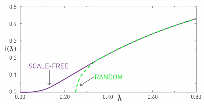Consider the above visual where the x-axis represents $\lambda = \frac{\beta}{\beta + \mu}$

Power-Law degree distribution
For networks with a power-law degree distribution ("scale-free network" curve shown in purple), and with an exponent $\gamma$ between 2 and 3, the variance (and the second moment) of the degree diverges to infinity ($\bar{k}^2 \rightarrow \infty$).

This means that the condition for an outbreak is

$\lambda > \bar{k} / \bar{k}^2 \rightarrow 0$

This is a remarkable result with deep and practical implications. It states that if the contact network has a power-law degree distribution with diverging variance, then any outbreak will always lead to an epidemic, independent of how small $\lambda$ is. Even a very weak pathogen, with a very small $\lambda$ , will still cause an epidemic.

SI,SIS,SIR under Arbitrary degree distributions¶

Here's a summary table for all three models

Computational Modeling of Epidemics¶

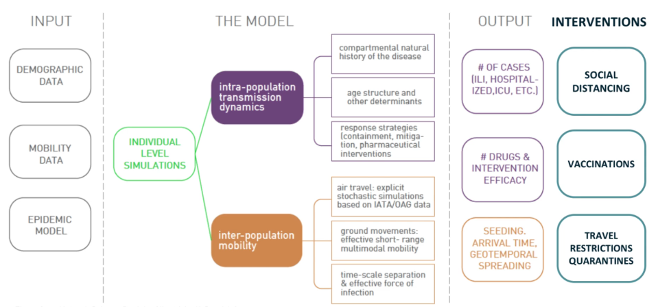
The mathematical models we studied earlier, are viable because they only depend on a few parameters and they provide clear insights. They are very simplified however, and they're based on very unrealistic assumptions. In practice, when public health agencies try to predict or mitigate the spread of an epidemic. They use more complicated models that can only be solved numerically.

As shown in the visualization for the gleam model developed by Northeastern University.

Effective Distance

Can we use geographical distance to predict the time that an epidemic will arrive at a state or country?

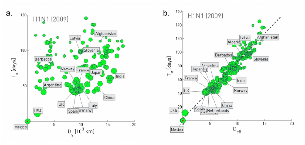
The plot at the left shows the geographic distance between Mexico and many other countries at the x-axis, while the y-axis shows the time that the H1N1 pandemic arrived in that country (defined as the number of days between the first confirmed case in that country and the beginning of the outbreak on March 17, 2009).

Clearly there is not any strong correlation between the two quantities.

Let us now define a different kind of distance, based on mobility data rather than geography:

Suppose that we have data from airlines, trains, busses, trucks, etc, showing how many travelers go from city i to city j.

The fraction of travelers that leave city i and arrive at city j is denoted by $p_{ij}$ .

The effective distance between the two cities is then calculated as $d_{i,j} = 1 - \ln p_{ij}$ .

The plot at the right replaces geographic distance with “effective distance”, and it shows that that the arrival day of this pandemic from Mexico was actually quite predictable based on strictly mobility data.

L10 Influence Phenomena On Networks¶

Objectives

Explain and analyze common models of influence on social networks
Select optimal “seed nodes” for maximum influence
Measure cascade phenomena on networks experimentally
Apply contagion modeling in practice, through case studies

“Word of mouth” is a powerful influence mechanism and it affects every aspect of our lives.

Think about behavior adoption: Do you like to exercise, eat healthy, party, smoke marijuana? It has been shown again and again that whether someone will adopt such behaviors or not mostly depends on his/her social network. And interestingly, it is not just strong contacts (such as family and close friends) that influence people. Our entire social network, including the crowd of acquaintances and indirect contacts that surround us, also have a strong effect on behavior adoption.

For centuries, the word-of-mouth mechanism required physical interaction between people. In the last few years, however, online social media such as Facebook, Twitter, or TikTok have provided us with the platform to influence not only the small number of people in our physical proximity – but potentially millions of people around the world.

YouTube or Twitter “influencers” today have tens of millions of followers – and it is often the case that their videos or tweets are being liked, commented on, or forwarded by millions of other people. Never before in the history of humankind, we found ourselves in the middle of so many sources of information (or misinformation), and never before every single one of us has at least the potential to influence pretty much any other person on the planet.

Diffusion, Cascades and Adoption Models¶

In sociology, a central concept is that of network diffusion. Given a social network and the specific node or nodes that act as the sources of some information, when will that information spread over the network?

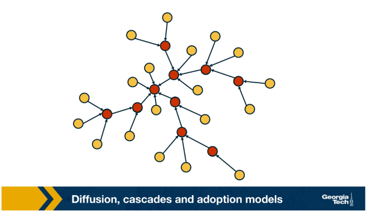
Which are the factors that determine whether someone will be influenced?
What is the total number of influenced people?
And how does that depend on the topology of the network?

Suppose that the network is an online social network such as twitter, and the edges points from follows to followees. In other words, the information flows in the opposite directions than the edges. Imagine that the node at the center of the network with six followers tweet something. That information is received by all of his or her follows but only three of them decide to retweet. Some of the followers of those three nodes also retweet. This creates a network cascade which is shown by the red nodes. In this example the size of the cascade is ten nodes and the depth of the cascade which is the largest distance from the source to any other node of the cascade is three hops. How can we describe such influenced phenomenon in a statistical framework?

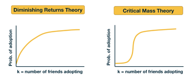
Theoretical models of influence:

two competing hypothesis
- diminishing returns theory
- and the critical mass theory
both postulate that the probability of adoption increases with the number of friends(direct social contacts) that have adopted the same information
diminishing returns theory, however, claims that this function is a concave function
critical mass theory claims that the adoption probability remains small until we exceed a certain threshold of adopting friends. And that it quickly saturates after we pass that threshold

As you can imagine, these two models produce very different results in many cases, regarding the size, and depth of cascades.

Empirical Findings About Cascades¶

Some general findings that have been observed repeatedly in the last few years in the context of different social networks and experiments of social influence.

For instance, an observational study of Twitter data analyzed 74 million tweet cascades that mention a URL. The tweets originated from 1.6 million “seed” users during a two-month period in 2009.

A first major observation is that the vast majority (90%) of tweets do NOT trigger a network cascade. They stop at the source. An additional 9% propagate only to one other user.

However, even though very few tweets trigger a significant network cascade, it is interesting that there are also tweets that cause major cascades, with a size that exceeds 1000 users and a depth of 8 or higher.

Linear Threshold Model¶

Consider a weighted (and potentially directed) network. The weight of the edge $w_{u,v}$ represents the strength of the relationship between nodes u and v. If the two nodes are not connected, we set $w_{u,v} = 0$.

The state of the node v can be inactive ($s_v = 0$) or active ($s_v = 1$)

Initially, the only active nodes are the sources of the cascade. In the context of social influence, for example, an inactive node may not be exposed to a certain behavior (e.g., smoking) or it may be that it has been exposed but it has not adopted that behavior.

Each node v has a threshold $\theta_v$. The Linear Threshold model assumes that a node v becomes active if the cumulative input from active neighbors of v is greater than the threshold $\theta_v$:

$\large s_v = 1 \text{ if } \sum_u s_u w_{u,v} > \theta_v$ Note that nodes can only switch from inactive to active once.
The Linear Threshold model is appropriate in diffusion phenomena when the ”critical mass” theory of social influence applies.

Question: if we only activate a certain node $v_0$, which are the nodes that will eventually become active? These nodes define the “activation cascade” of $v_0$. Note that this cascade may cover the whole network, may include only $v_0$, or it may be somewhere in between. Of course, the cascade of $v_0$ includes nodes that are reachable from $v_0$.

One simplification of the linear threshold is the homogenous case in which all nodes have the same threshold $\theta_v$.

Other variations of the model include one in which two behaviors A and B are spreading at the same time, meaning that the state of a node can take three different values (inactive, A and B). In that case, the state of a node can switch between states A and B over time.

Another common variation is the “Asynchronous Linear Threshold” model. In that case, each edge has a certain delay. This means that different nodes can become active at different times.

The edge delays can affect the temporal order in which nodes join the activation cascade – but they cannot change the size of the cascade. We will review an application of this model on brain networks at the end of this lesson.

Independent Contagion Model¶

In some cases the activation of a node v can be triggered by a single active neighbor of v, independent of the state of other neighbors of v. The Independent Contagion model is more appropriate in such problems.

Again, the state of each node can be inactive or active. If there is an edge from u to v, then the weight $w_{u,v}$ of the edge in this model represents the probability that node u activates node v when the former becomes active.

Note that node u has a single chance to activate node v. Nodes stay in the active state after they have been activated.

An important difference with the Linear Threshold model is that the Independent Contagion model is probabilistic, and so the activation cascade of a seed node v has to be described statistically.

Deffuant Model For Opinion or Consensus Formation¶

In some cases, it is a gross oversimplification to represent the state of each node as a binary variable (active vs inactive). Instead, we need a scalar to represent the state of each node. For example, our opinion about the risk of a potential COVID-19 infection may vary anywhere between the two extremes “I am extremely worried” to “I do not care at all”. Typically, our opinion about such matters depends on the opinion of our social contacts.

The Deffuant model of opinion (or consensus) formation assumes that the state of a node v at time t is a scalar $s_v(t)$ that falls between 0 and 1.

A key parameter of the model is the “tolerance threshold” $\delta$:

If the state of two connected nodes, say u and v, is greater than the threshold $\delta$: $|s_v(t) - s_u(t)| \ge \delta$, the two neighbors “disagree” so strongly that they do not influence each other, and their state remains as is.
Otherwise, if $|s_v(t) - s_u(t)| \lt \delta$, then they influence each other, changing their state at the next time instant as follows:
$s_v(t+1) = s_v(t) + \mu[s_u(t) - s_v(t)]$
- and
$s_v(t+1) = s_v(t) - \mu[s_u(t) - s_v(t)]$
- where $\mu$ is the convergence parameter of the model.
for $\mu$=1/2 the two states will become identical at t+1.
In general $0 < \mu < 0.5$, just in case they won't reach agreement

The model proceeds iteratively, by selecting a randomly chosen pair of neighbors in each iteration. If the network is weighted then the order at which pairs of nodes interact may depend on the weight of the corresponding edge. Note that whether two neighbors influence each other or not may change over time.

For example, consider the network shown in the visualization ($\mu$=1/2, $\delta$=0.45). Suppose that we select pairs of neighboring nodes in the following order:

x and z: their opinion converges to $s_x = s_z = 0.15$
u and v: their opinion converges to $s_x = s_z = 0.6$
u and z: their opinion does not change
v and y: their opinion converges to $s_x = s_z = 0.6$

At that point, the opinion of every node has converged to a final value because any pair of adjacent nodes either have the same opinion, or their opinion differs by more than the threshold $\delta$.

Game Theoretic Diffusion Models¶

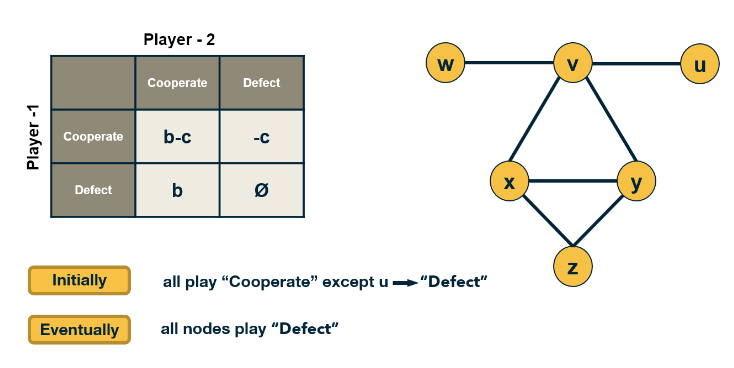
In some cases, the behavior of nodes in a social network can be captured more realistically with game-theoretic models: where each node is a player that chooses rationally between a set of strategies. Crucially, the “payoff” of each strategy for player v also depends on the strategies chosen by the neighbors of v.

Let's consider a simple co-ordination game. Each player can choose to either “Cooperate” (work with others) or “Defect” (act selfishly). Co-operating with a neighbour player comes at a cost c. If two players co-operate they will both recieve benefit b. We can quickly see that it makes sense to co-operate when b > c.

However some players may choose to Defect. In that case, they get the benefit b from every Cooperator they interact with – and they do not pay any cost. Think of the “friend” that will borrow things from you but he/she would never lend you anything.

Each player interacts only with its neighbors. Further, when a player chooses a strategy (say to be a Cooperator), that strategy applies to all bilateral interactions with its neighbors.

So, if player v has k connections, and m of those neighbors are Cooperators, then if v chooses to be a Cooperator its payoff will be bm - ck. It obtains a benefit b from each neighbor, but pays an additional penalty c for every connection. If it chooses to be a Defector, its payoff will just be bm.

If a node is surrounded by Cooperators, then it would benefit in the short-term by becoming a Defector. But its neighbors would also decide to do the same, and they would all become Defectors. So eventually, the payoff of all players will be lower than if they had all remained Cooperators.

This illustrates how selfish behavior may quickly spread on a network, even if it is harmful to everyone in the long term.

Seeding for Maximum Network Cascade¶

An important problem in the context of network diffusion is how to select a subset of k nodes that if activated, can collectively create the largest network cascade. In the context of marketing for instance, an advertising company may want to promote a certain product through an online social network, such as facebook.

Suppose that they can give the product for free to k users, they expect that these k users will then influence their neighbors, online friends to buy the same product and also influence their own friends, creating a network cascade. obviously, the marketing company would like to select the set of k nodes that can cause the maximum sites cascade.

Mathematically this can be stated as a constrained optimization problem. We are given a weighted and potentially directed network and a diffusion model such as the linear threshold or the independent cascade model.

we are given a weighted and potentially directed network, as well as a diffusion model
Let S be the nodes that are initially active
- f(S) represents the set of nodes that will eventually become active , including S
- f(S) is referred to as the cascade size of S

Let S be a set of nodes thast we initially activate, the sources in other words. f(S) represents the set of nodes that will eventually become active, including those in S. After the cascade, f(S) is referred to as the cascade size that started from the sources S. The objective here is to select set S such that f(S) is maximum subject to the constraint that the size of S is at most k nodes. When the network diffusion model is probabilistic such as the independent cascade model, the objective is to maximize the expected value of f(S).

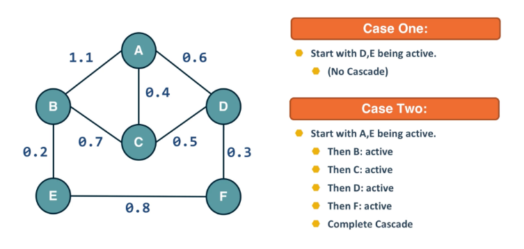
The visualization here shows two cases when k is equal to 2. In the first case, we initially activate nodes D and E and the cascade does not extend beyond those two nodes. In the second case, we activate initially nodes A and E. Here, the cascade eventually covers the whole network.

Submodularity of Objective Function¶

The function we try to maximize, f(S), is nonlinear and it obviously depends on the topology of the network as well as on the specific diffusion model. Furthermore, the function has an interesting property referred to as “submodularity”.

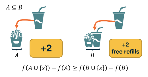
Defining Submodularity: Suppose that a function f(X) maps a finite subset X of elements from a ground set U to non-negative real numbers.

The function f(X) is called monotone if $f(v \cup X) \ge f(X)$ for any $v \in U$ and any subset X.
The function f(X) is called submodular if it satisfies the following “diminishing returns” property:
- $f(v \cup X) - f(X) \ge f(v \cup T) - f(T)$ for any subsets X and T of U such that $X \subset T$

In other words, the marginal gain from adding an element v to a set X is at least as high as the marginal gain from adding the same element to a superset T of X.

The bad news: optimizing such functions, subject to the constraint that X includes k elements, is an NP-Hard problem, and so it cannot be solved efficiently by any algorithm (unless if P = NP).

The good news: Consider an iterative greedy heuristic that adds one element in X in each iteration, selecting the element that gives the maximum increase in f(X). This simple algorithm has an approximation ratio (1 - 1/e). This means that the greedy solution cannot be worse than about 63% of the optimum value of f(X).

What this means is that, even though the greedy algorithm is suboptimal, we have a reasonable bound on its distance from the optimal solution.

Monotone and Submodular Function¶

Now that we know how to optimize, at least approximately, monotone and submodular functions, we can go back to the problem of maximizing network diffusion. Suppose that S is one or more initially active nodes, and $g(S)$ is the resulting cascade of active nodes. Is the cascade function $g(S)$ monotone and submodular? The fact that the cascade size is monotone is obvious: if we increase the number of initially active nodes, we cannot decrease the size of the cascade. It is also possible to show that the cascade size is a submodular function, for both the Linear Threshold and the Independent Cascade model. Let us focus on the latter here.

With the Independent Cascade model, we can first randomly choose for every edge of the network whether it is “live” or ”blocked”, based on its activation probability.

The set of live edges for such a specific random assignment can then be used to determine the set of active nodes at the end of the cascade.

The important point is that a node w will be part of the cascade if and only if there is a path of live edges from the initially active node(s) to w.

To prove the submodularity of the cascade size, we need to show that the number of NEW nodes that become active after we add a node v in the set of active nodes is larger for S than for its superset T.

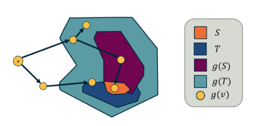
Please refer to the above diagram. S is a subset of T, and $g(S)$ and $g(T)$ are the corresponding sets of active nodes.

There are two cases:

The new nodes that become active after the activation of $v$ are neither in $g(S)$ nor $g(T)$
the new active nodes are in $g(T)$ but not in $g(S)$. Note that the inverse cannot be true (in g(S) but not g(T))

So, more nodes are activated when $v$ is added to $S$ compared to when $v$ is added to $T$.

The previous argument holds for the random assignment of live edges we started from.To show that the expected value of the cascade size is also submodular, we need to use the fact that: if a set of functions $f_1,f_2,\cdots$ are submodular, then any non-negative linear combination of those functions is also submodular (non-negative because the scaling coefficients are probabilities).

Cascades in Networks with Communities¶

We have already established in earlier lessons that most real-world networks have clusters of strongly connected nodes that we refer to as communities. How do such communities affect the extent of diffusion processes, such as those discussed earlier in this lesson? Is it that the community structure facilitates or inhibits the diffusion of information on networks?

To make this analysis more concrete, let us start with a quantitative definition of a network community structure:

We say that a set of nodes C forms a cluster (or community) of density p if every node in that set has at least a fraction p of its neighbors in the set C.

The visualization shows three such clusters of nodes, each of them containing four nodes, with density p=2/3.

Suppose that we model the diffusion process with the Linear Threshold Model. To keep things simpler, let us consider the homogeneous version of this model in which all edge weights are the same.

If the threshold is $\theta$ then a node becomes active if and only if at least a fraction $\theta$ of its neighbors are active.

The visualization shows an example in which the cascade starts from two nodes (nodes 7 and 8). If the threshold $\theta$ is larger than 2/3, the cascade will not expand beyond those initial nodes.

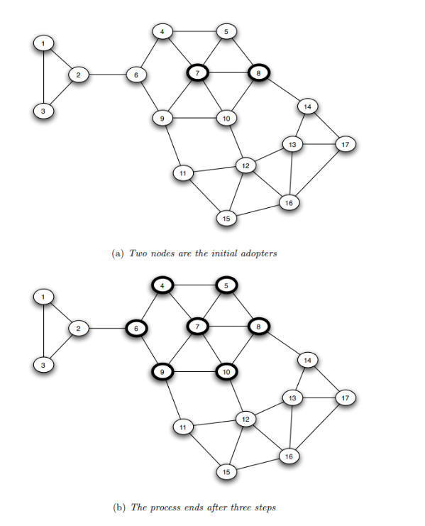
If $\theta = 2/5$, then the cascade in this example will expand to the seven nodes that are highlighted within 3 steps. In the first step, nodes 5 and 10 will become active. In the second step, nodes 4 and 9 will become active. And in the third step, node 6 will become active. The cascade will stop at that point.

Note that these 7 highlighted nodes form a cluster of density p=2/3.

Is there a relation between the density of the cluster p, and the maximum value of the activation threshold that is required for the establishment of a complete cascade in the network?

This is the main result we will establish on the next page.

Dense Clusters Affect Cascades?¶

We will first prove the following result:

Suppose that we model the diffusion process using the Linear Threshold Model with threshold value $\theta$.

If the set of initially active nodes is A, then the cascade will NOT cover the whole network if the network includes a cluster of initially inactive nodes with density greater than $1 - \theta$.

Proof: We will prove this by contradiction

Consider such a cluster of initially inactive nodes with density greater than $1 - \theta$. Assume the opposite of what we want to prove, i.e., that one or more nodes in this cluster eventually become active. Let v be the first such node in the cluster.

At the time v became active, its only active neighbors could be outside the cluster. But since the cluster has density greater than $1 - \theta$, at least a fraction of v’s neighbors are in the cluster. So, less than a fraction $\theta$ of v’s neighbors are outside the cluster. Even if all of those neighbors were active, that would not be enough to activate v. This leads to a contradiction, and so it cannot be that the cluster eventually includes an active node.

Moreover, we can show the following related result:

If a network cascade that starts from a set of initial nodes A does not cover the whole network, then the network must include a cluster of density greater than $1 - \theta$.

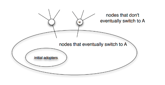
Asynchronous Linear Threshold (ALT) Model¶

The unweighted Linear Threshold model assumes that a “node” (brain region in this case) becomes active when more than a fraction of the neighboring nodes it receives incoming connections from being active.

Here, we use a variation of this model with

weighted connections, where the weights are based on the connection density of the projections, and
connection delays, where the delays are based on the physical distance between connected brain regions.

The state of a node-i is initially $s_i(t) = 0$. It becomes equal to 1 when:

$ \large \sum_{j\in N_{in}(i)} w_{ji} s_j(t - t_{ji}) > \theta$
Where $N_{in}(i)$ is the set of nodes that node-i recieves incoming connections from.
$w_ji$ and $t_ji$ are the weights and the delay of the connection from node-j to node-i, respectively
and $\theta$ is the activation threshold

The ALT model is simple yet it incorporates information about distances between brain regions (to model connection delays) and uses local information (a thresholding nonlinearity) to potentially gate the flow of information.

The above visualization shows a toy example with five nodes. The source of the cascade is node $n_1$. Each edge shows two numbers, the first is its delay, and the second is its weight. The activation threshold is set to $\theta = 1$. The cascade takes 7-time units to propagate throughout the whole network.

L11 Other Dynamic Processes Of/On Networks¶

Objectives

Understand the notion of network robustness in the context of random failures and attacks
Learn about the problem of distributed search and how its efficiency depends on the network structure
Model distributed synchronization phenomena on networks
familiar with adaptive or co-evolutionary network phenomena

Inverse percolation on Grids and G(n,p) Networks¶

Suppose we have a dynamic network under a dynamic process where the topology changes over time. For instance nodes may be removed and/or added as time goes on. This happens often in practice as a result of failures (e.g., Internet router malfunctions, removal of species from an ecosystem, mutations of genes in a regulatory network) or deliberate attacks (e.g., destroying specific generators in the power distribution network, arresting certain people in a terrorist network).

Further suppose we look at the simplest case in which instead of a network we have a two-dimensional grid, and a node is placed at every grid point. Two nodes are connected if they are in adjacent grid points.

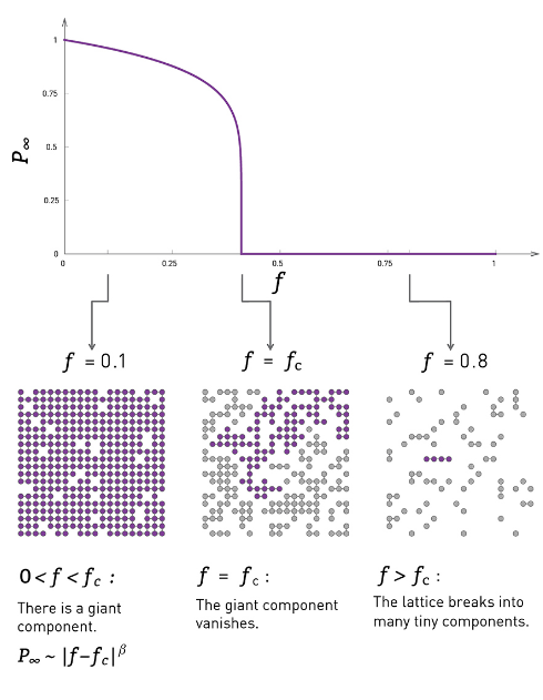
In the context of random failures, we can select a fraction f of nodes and remove them from the grid, as shown in the visualization above. The y-axis in that visualization shows the probability that a randomly chosen node belongs in the largest connected component on the grid.

When f is low, the removals will not affect the grid much in the sense that most of the remaining nodes still form a single, large connected component (referred to as giant component). As f increases however the originally connected grid will start “breaking apart” in small clusters of connected grid points. Further, as the visualization shows, this transition is not gradual. Instead, there is a sudden drop in the size of the largest connected component as f approaches (from below) a critical threshold $f_c$. At that point the giant component disappears, giving its place to a large number of smaller connected components.

In physics, this process is referred to as inverse percolation and it has been extensively studied for both regular grids as well as random G(n,p) networks.

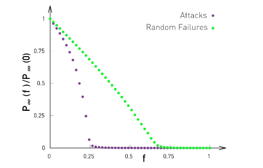
The visualization at the left shows simulation results of a G(n,p) network with n=10,000 nodes and average degree $\bar{k}=3$.

The y-axis shows, again, the probability that a node belongs in the largest connected component of the graph after we remove a fraction f of the nodes, normalized by the same probability when f=0. In the case of random failures, note that the critical threshold $f_c$ is about 0.65-0.70. After that point, the network is broken into small clusters of connected nodes and isolated nodes. The same plot also shows what happens when we attack the highest-degree nodes of the network. We will come back to this later in this Lesson.

Next we will see an animation for power-law networks, in which the degree distribution has infinite variance. In that case, the process of random node removals behaves very different than the process of node attacks.

Then, after that animation, we will derive and show some mathematical results for the critical threshold –for the case of random failures as well as for the case of higher-degree node attacks.

Random Removals (Failures) vs Targeted Removals (Attacks)¶

We consider two ways of removing nodes from a network, random removals or failures, and targeted removals of the highest degree nodes. We refer to those as attacks. Imagine a network, with 50 nodes and about 100 edges, created with the preferential attachment model, and so, that the degree distribution is approximately a power law with exponent 3 as we learn in lesson four. Note that the size of its node is proportional to its degree.

Random removals: in iteration, we select a random node and remove it, This changes the degree of all nodes connected to the remove node. The question we focus on is: how many nodes do we need to remove until the network’s largest connected component folds apart to just a small fraction of the initial network size?

This should happens after we remove about 40 to 45 out of the 50 nodes. There may be four to five hubs keep the network connected because of the remaining connections. The largest connected component breaks down, only when we have removed so many nodes, but the original hubs are no longer high degree nodes.

Targeted removals or attacks: what happens if we remove the node with the highest degree in each iteration. Such an attack on the network would require that the attack has some information about the topology of the network, or the degree of its node. In this case, it takes only the removal of about 10 nodes before the largest connected component falls apart to disconnected individual nodes, and few small connected components.

The qualitative conclusion from these two animation is that the networks with power law degree distribution, and that’s with hubs are quite robust to random failures but they are also very vulnerable to targeted attacks on their highest degree nodes.

Molloy-Reed Criterion¶

If the largest connected component (LCC) of a network covers almost all nodes, we refer to that LCC as the giant component of the network.

To derive the critical threshold of an inverse percolation process, we need a mathematical condition for the emergence of the giant component in a random network (including power-law networks). This condition is referred to as Molloy-Reed criterion (or principle): Consider a random network that follows the configuration model with degree distribution p(k) (i.e., there are no degree correlations). The Molloy-Reed criterion states that the average degree of a node in the giant component should be at least 2.

Intuitively, if the degree of a node in the LCC is less than 2, that node is part of the LCC but it does not help to expand that component by connecting to other nodes. So, in order for the LCC to expand to almost all network nodes (i.e., in order for the LCC to be the giant component), the average degree of a node in the LCC should be at least two.

To express the Molloy-Reed criterion mathematically, let us first derive the average degree of a node in the LCC, as follows:

Suppose that j is a node that connects to the LCC through an LCC node i.
Let $P[k_j = k | A_{i,j} = 1]$ be the probability that node j has degree k, given that nodes i and j are connected.
From Bayes we get
- $\large P[k_j = k | A_{i,j} = 1] = \frac{ P[k_j = k] P[A_{i,j} = 1 | k_j = k] }{P[A_{i,j} = 1]}$
for a network with n-nodes and m-edges the denominator is
- $\large P[A_{i,j} = 1] = \frac{2m}{n(n-1)} = \frac{\bar{k}}{(n-1)}$
- where $\bar{k}$ is just the average degree
Further more
- $P[A_{i,j} = 1 | k_j = k] = k / (n-1)$
- because j chooses between n-1 nodes to connect to with k edges
putting the together and back into the bayes formulas yields and average degree of nodes in the LCC as
- $\large \sum_k k P[k_j = k | A_{i,j} = 1] = \frac{\bar{k^2}}{\bar{k}}$

We can restate the Molly-Reed criterion in mathematical terms as follows:

In a random network that follows the configuration model with degree distribution p(k), if the first and second moments of the degree distribution are $\bar{k}$ and $\bar{k^2}$ respectively,
- the network has a giant connected component if
- $\large \frac{\bar{k^2}}{\bar{k}} \ge 2 $

Robustness of Networks to Random Failures¶

We will now present the critical threshold under random node failures. The detailed proof of this result can be found in the textbook (Advanced Topics 8.C).

The key points of the proof however are the following:

A. When we remove a fraction f of the nodes, the degree distribution changes. A node that had degree k in the original network, will now have a degree k_1 < k with probability
- ${k \choose k_1} f^{k-k_1} (1-f)^k$
- because each of the ${k-k_1}$ neighbors of that node is removed with probability f, and there are ${k \choose k_1}$ ways to choose $k_1$ from k neighbors.
B. If the probability that a node has degree k in the original network is $p_k$, the probability that the node has degree $k_1$ in the reduced network (the network that results after the removal of a fraction f of the nodes) is:
- $p'_k = \sum_{k = d_1} p_k {k \choose k_1} f^{k-k_1} (1-f)^k $
C. The average degree of the reduced network is a fraction (1-f) of the average degree of the original network:
- $\bar{k} = (1-f) \bar{k}$
D. Similarly, the second moment of the degree distribution of the reduced network is:
- $\bar{k^2} = (1-f)^2 \bar{k^2} f(1-f) \bar{k}$
- where $\bar{k^2}$ is the second moment of the degree distribution

Recall the Molly-Reed criterion: $\frac{\bar{k^2}}{\bar{k}} \ge 2 $

we can sub the above expressions into MR to get
- $\large f_c = 1 - \frac{1}{ (\bar{k^2} / \bar{k} ) -1 }$

G(n,p)

For G(n,p) deg variance is equal to avg degree so $\bar{k^2} = \bar{k}(\bar{k}+1)$
- $\large f_{c,G(np)} = 1 - \frac{1}{ \bar{k} }$
- So, if the average degree of a large G(n,p) network is 2, we expect that the giant connected component of the network will disappear when the fraction of removed nodes exceeds about 50%

Power-Law Networks
What happens with power-law networks in which the degree exponent is between 2 and 3? As we saw in Lesson-4, in that case the first moment is finite but the degree variance and the second moment diverge. So, $f_c$ converges to 1, at least asymptotically,

$\large f_{c,2<\gamma<3} \rightarrow 1$

This is a remarkable result that needs further discussion: it means that such networks stay connected in a single component even as we remove almost all their nodes. Intuitively, this happens because networks with diverging degree variance have hubs with very large degree. Even if we remove a large fraction of nodes, it is unlikely that we remove all the hubs from the network, and so the remaining hubs keep the network connected.

The situation is not very different if we randomly remove links instead of nodes, as shown in Figure (b). Here, we remove a fraction f of all links in the network. It can be shown that the network’s giant connected component disappears at the same critical threshold as in the case of node removals. The visualization in Figure (b) refers to a G(n,p) network in which n=10,000 nodes and the average degree is $\bar{k}=2$. As predicted by the critical threshold equation, the giant component disappears when we remove 1-(1/2)=50% of all edges. For lower values of f, the effect of random node removals is more detrimental than the effect of random link removals (why?).

What happens with power-law networks in which the degree exponent $\gamma$ is larger than 3? In that case the degree variance is finite, and so we can use the critical threshold equation to calculate the maximum value of f that does not break the network’s giant component. Figure (c ) shows numerical results of three values of $\gamma$, the network size is n=10,000 and the minimum node degree $k_{min} = 2$.

Robustness of Networks to Attack¶

Let us start with some simulations. Figure (a) contrasts the case of random failures and attacks in a G(n,p) network with n=10,000 nodes and average degree $\bar{k}=3$. The y-axis shows, as in the previous page, the probability that a node belongs in the largest connected component of the graph after we remove a fraction f of the nodes, normalized by the same probability when f=0. In the case of random failures, the critical threshold $f_c$ is about 0.65-0.70 – the theoretical prediction for an infinitely large network is $1 - 1/\bar{k} = 2/3$.

The same plot shows what happens when we “attack” the highest-degree nodes of the network. Specifically, we remove nodes iteratively, each time removing the node with the largest remaining degree, until we have removed a fraction f of all nodes.

This “attack” scenario destroys the LCC of the network for an even lower value of f than random removals. The critical threshold for attacks is about 0.25 in this network. The fact that the critical threshold for attacks is lower than for random failures should be expected – removing nodes with a higher degree makes the LCC sparser, increasing the chances that it will be broken into smaller components.

As we know from Lesson-4 however, G(n,p) networks do not have hubs and the degree distribution is narrowly concentrated around the mean (Poisson distribution). What happens in networks that have hubs – and in particular what happens in power-law networks in which the degree variance diverges?

Figure (b) contrasts random failures and attacks for a power-law network n=10,000 nodes, degree exponent $\gamma = 2.5$, and minimum degree $k_{min}=1$. Even though the case of random failures does not have a critical threshold ($f_c$ tends to 1 as the network size increases), the case of attacks has a critical threshold that is actually even lower (around 0.2 in this example) than the corresponding threshold for G(n,p) networks. Power-law networks have hubs, and attacks remove the hubs first. So, as the network’s hubs are removed, the giant component quickly gets broken into many small components.

The moral of the story is that even though power-law networks are robust to random failures, they are very fragile to attacks on their higher degree nodes.

The mathematical analysis of this attack process is much harder (you can find it in your textbook in “Advanced topics 8.F”) and it does not lead to a closed-form solution for the critical threshold $f_c$.

Specifically, if the network has a power-law degree distribution with exponent $\gamma$ and with minimum degree $k_{min}$, then the critical threshold $f_c$ for attacks is given by the numerical solution of the equation:

$\large f_c^{\frac{2-\gamma}{1-\gamma}} = 2 + \frac{2-\gamma}{3-\gamma} k_{min} ( \frac{3-\gamma}{1-\gamma} - 1 )$

Figure (c ) shows numerical results for the critical threshold as a function of the degree exponent $\gamma$, for two values of $k_{min}$, and separately for failures and attacks.

The key points from this plot are:

In the case of random failures, $f_c$ decreases with $\gamma$ this is expected because as $\gamma$ decreases towards 3, the degree variance increases, creating hubs with higher-degree.
In the case of attacks, however, the relation between $f_c$ and $\gamma$ is more complex, and it also depends on $k_{min}$. In the case of $k_{min}=3$, as $\gamma$ decreases, $f_c$ decreases because the degree variance increases, the hubs have an even greater degree, and removing them causes more damage in the network’s giant component.
As expected, for given values of $\gamma$ and $k_{min}$, attacks always have a smaller $f_c$ than random failures.
As $\gamma$ increases, and for a given value of $k_{min}$, the critical threshold $f_c$ for attacks approaches the critical threshold for random failures. The reason is that as $\gamma$ increases, the variance of the degree distribution decreases. In the limit, the degree variance becomes zero and all nodes have the same degree. In that case, it does not matter if we remove nodes randomly or through attacks.

Small-world Networks and Decentralized Search¶

Back in the late 60s, the famous sociologist Stanley Milgram, decided to study the small world phenomenon. Until then, this was only a fascinating anecdote. People would find it amusing every time it was discovered that two random individuals know hte same person. Nobody had studied this empirically however, and the six degrees fo separation principle was just an expression.

Milgram asked several individuals in Nebraska to forward the letter to a target person in Boston. He gave participants the name, address, and occupation of the target. But the participants could not just send the letter directly to the target. They had to forward the letter to a person they knew on a first name basis with a goal of reaching the target as soon as possible. Most participants chosen acquaintances based on geographical and occupational information. It is reasonable to expect that these letters would never reach their destination. Because finding such a path between two random individuals, one in Nebraska and another in Boston would require a very long number of intermediates. Besides, it could be that even if there are short paths between these two individuals, their immediate people would not know that short path exists.

And so the letters would keep getting forwarded in the vicinity of the target but never actually reaching the target. Surprisingly, one third of the letters made it to the target. The histogram that you see here from Milgram original paper shows that the median distance was six steps just as the six degree of separation principle detected.

What can we learn Stanley Milgram’s small world experiment? What does it reveal about the structure of hte underlying social network? And what does it say about the efficiency of a distributed search process in small-world-networks? These are questions that we answer in the next few pages using an elegant mathematical model that was developed by John Kleinberg at Cornell University.

Decentralized Search Problem¶

Milgram’s experiment has been repeated by others, both in offline and online social networks. These studies show two points:

Even global social networks (Facebook has around one billion users) have multiple short paths to reach almost anyone in the network (typically around 5-6 hops, and almost always less than 10 hops).
It is possible to find at least one of these short paths with strictly local information about the name and location of your neighbors, without having a global “map” (topology) of the network – and without a central directory that stores everyone’s name and location in the network.

The first point should not be surprising to us by now. Recall what we learned about Small World networks in Lesson-5. A network can have both strong clustering (i.e., many triangles, just as a regular network) and short paths (increasing logarithmically with the size of the network, just as G(n,p) networks). The way this is achieved in the Watts-Strogatz model is that we start from a regular network with strong clustering and rewire a small fraction (say 1%) of edges to connect two random nodes. These random connections connect nodes that can be anywhere in the network – and so for large networks, these random connections provide us with “long-range shortcuts”. If you do not recall these points, please review Lesson-5.

Let us now focus on the second point: how is it possible to find a target node in a network with only local information, through a distributed search process? First, let us be clear about the information that each node has: a node v knows its own location in the network (in some coordinate system), the locations of only the nodes it is connected to, and the location of the target node.

The metric we will use to evaluate this distributed search process is the “expected delivery time”, i.e., the expected number of steps required to reach the target, over randomly chosen source and target nodes, and over a randomly generated set of long-range links.

To answer the previous question, we will consider an elegant model developed by Jon Kleinberg. Suppose that we start with a regular grid network in k-dimensions (the visualizations shown refer to k=2 but you can imagine mesh networks of higher dimensionality). Each node is connected to its nearest neighboring nodes in the grid. Note that this network does not have cliques of size-3 (triangles) but it still has strong clustering in groups of nodes that are within a distance of two hops from each other.

Let $d(v,w)$ be the distance between nodes v and w in this grid. Kleinberg’s model adds a random edge out of v, pointing to a node w with a probability that is proportional to $d(v,w)^{-q}$ – the exponent q is the key parameter of the model as we will see shortly.

The value of q controls how “spread out” these random connections actually are. If q=0, the random connections can connect any two nodes, independent of their distance (this is the case in the Watts-Strogatz model) – and so they are not very useful in decentralized search, when you try to “converge” to a certain target in as few steps as possible. If q is large, on the other hand, the random connections only connect nearby nodes – and so they will not provide the long-range shortcuts that are necessary for Small World property.

Optimal Search Exponent in Two Dimensions¶

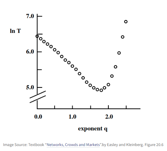
Let us start with some simulation results. The plot shows the exponent q at the x-axis, when the initial grid has k=2 dimensions. The y-axis shows the logarithm of the expected delivery time in a grid with 400 million nodes. Each point is an average across 1000 runs with different source-target pairs and different assignments of random edges.

As expected, values of q that are either close to 0 or quite large result in very slow delivery times. The random edges are either ”too random” (when q is close to 0) or ”not random enough” (when q is large).

It appears that the optimal value of the exponent q is when it is close to 2 – which, remember, is also the value of the dimension k in these simulations. Is this a coincidence?

The answer is that we can prove that the optimal value of q is equal to k. In other words, if we want to maximize the speed of a decentralized search in a k-dimensional world, we should have random “shortcut links” the probability of which decays as $d(v,w)^{-k}$ with the distance between two nodes. This surprising result was proven by Kleinberg in 2000.

The proof, for k=1 and 2, is in in the online textbook “Networks, Crowds and Markets” by Easley and Kleinberg (section 20.7).

Next, Lets build some basic intuition behind this result.

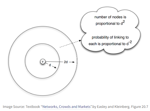
We can organize distances into different “scales of resolution”: something can be around the world, across the country, across the state, across town, or down the block.

Suppose that we focus on a node v in the network – and consider the group of nodes that are at distances between d and 2d from v in the network, as shown in the visualization. If v has a link to a node inside that group, then it can use that link to get closer to the set of nodes that are within that scale of resolution.

So, what is the probability that v has a link to a node inside that group? And how many nodes are expected to be in that distance range?

In a two-dimensional world, the area around a certain point (node v) grows with the square of the radius of a circle that is centered at v. So, the total number of nodes in the group that are at a distance between d and 2d from v is proportional to $d^2$.

On the other hand, the probability that node v links to any node in that group scales as $d(v,w)^{-2}$, when $q=k=2$. So, if node w is at a distance between d and 2d from v, the probability that it is connected to v is proportional to $d^{-2}$.

Hence, the number of nodes that are at a distance between d and 2d from v, and the probability that v connects to one of them, roughly cancel out. This means that the probability that a random edge links to a node in the distance range [d,2d] is independent of d.

In other words, when q=k=2, the long-range links are formed in a way that “spreads them out” roughly uniformly over all different resolution scales. This is the key point behind Kleinberg’s result.

If the exponent q was lower than k=2, the long-range links would be spread out non-uniformly in favor of larger distances, while if q was larger than k=2, the long-range links would be spread out non-uniformly in favor of shorter distances.

Decentralized Search In Practice¶

In the last few years, researchers have also investigated the efficiency of decentralized search empirically, mostly doing experiments in online social networks. There are a number of practical issues that have to be addressed however when we move from Kleinberg’s highly abstract model to the real world.

First, in practice, people do not “live” on a regular grid. In the US, for instance, the population density is extremely nonuniform, and so it would be unreasonable to expect that the q=k=2 result would also hold true about real social networks. One way to address this issue is to work with “rank-based links” rather than “distance-based links”. The rank of a node w, relative to a given node v, is the number of other nodes that are closer to v than w – see Figure (a).

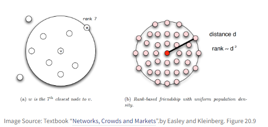
We can now modify Kleinberg’s model so that the random links are formed based on node ranks, rather than rank distances. In Figure (b), we see that when nodes have a uniform population density, a node w at distance d from v will have a rank that is proportional to $d^2$, since all nodes inside a circle of radius d will be closer to v than w.

In fact, it can be proven that, for any population density – not just uniform – if the random links are formed with a probability that is proportional to 1/$rank_v(w)$, the resulting network will have minimum expected delivery time – note that the exponent, in this case, is 1, not 2.

This result has been empirically validated with social experiments on an earlier social networking application called LiveJournal – but similar experiments have been also conducted on Facebook data. Figure-c shows the probability of a friendship as a function of geographic rank on the blogging site LiveJournal. Note that the decay is almost inversely proportional to the rank.

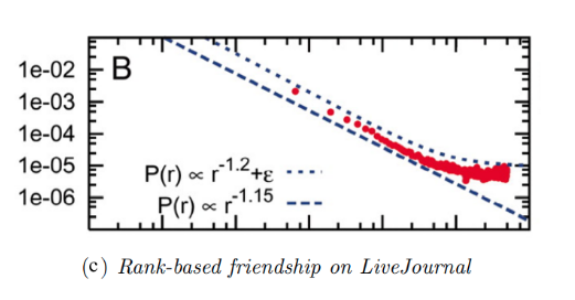
Another way to generalize decentralized network search is by considering that people can belong to multiple different groups (family, work, hobbies, etc), and so the distance (or rank) between two network nodes can be defined based on the group at which the two nodes are closest. This group is referred to as the ”smallest focus” that contains both nodes. This generalized distance metric has allowed researchers to examine more realistically whether real social networks have the optimal “shortcut links” to minimize the delivery time of the decentralized search, in terms of the corresponding exponent.

An interesting question, that is still largely an open research problem, is: why is it that real social networks, both offline and online, have such optimal “shortcut links”? Clearly, when people decide who to be friends with on Facebook or in real life, they do not think in terms of distances, ranks, and exponents!

One plausible explanation is that the network is not static – but instead, it evolves over time, constantly rewiring itself in a distributed manner, so that searches become more efficient. For instance, if you find at some point that you want some information about a remote country (e.g., Greece), you may try to find someone that you know from that country (e.g., the instructor of this course) and request that you get connected on Facebook. That link can make your future searches about that country much more efficient.

Synchronization of Coupled Network Oscillators¶

Synchronization is a very important property of both natural and technological system. In broad terms, synchronization refers to any phenomenon in which several distinct but coupled, dynamic element have a coordinated dynamic activity. For example, all the devices that are connected to the internet have synchronized clock using a distributed protocol called NTP, network time protocol. Interestingly, this protocol works quite well despite the fact that internet delays are unknown and time varying and the complete topology of the internet is not known.

A classic example of emergent synchronization is shown in this youtube video. Five metronomes are placed on a moving bar so that the motion of its metronome is loosely coupled with the motion of others. The metronomes start from a random phase and under certain conditions that we discuss later in this lesson, they can get completely synchronized after some time as this video shows. Note that in this case, the communication between the five dynamic elements is only indirect.

The metronomes do not exchange any messages, instead, each of them affects to a small degree, the movement of the underlying board and that board affects hte movement of every metronome. Another example of self organized synchronization in nature is when many fireflies gather close together as this image shows. Note that each firefly cannot see all other fireflies such global communication is not necessary in synchronized systems. Instead, the remarkable effect is that a large number of systems can get synchronized at least a period of time even if each of them can only communicate locally with other nearby systems.

Similar distributed synchronization phenomena also take place with flock of birds, and school of fish, forming fascinating dynamic patterns. In technology, similar problems emerge when we have a group of robots, autonomous vehicles or drones that need to coordinate without having a centralized controller. Our brains also rely on short term synchronization between thousands of neurons, so that different brain regions can communicate. This type of synchronization, referred to as coherence is shown at this video.

The video shows three views from the lateral and dorsal of the zebrafish brain using calcium imaging. Whenever a cluster of neurons fires, the corresponding part of hte brain lights up. Note how different brain regions get active at about the same time, occasionally producing large avalanches of neural activity throughout most of the brain. Synchronization is not always a desirable state, however. For example, too much synchronization in the brain can cause seizures. This image shows EGG recordings during the onset of an epileptic seizure. The scissor start at about the middle of the blood, and it shows major waves discharges at the Frequency of about three hertz over most of the patient’s cortical surface.

Coupled Phase Oscillators – Kuramoto Model¶

Collective synchronization phenomena can be complex to model mathematically. The class of models that have been studied more extensively focuses on coupled phase oscillators.

Suppose that we have a system of N oscillators. The j’th oscillator is a sinusoid function with angular frequency $\omega_j$. To simplify suppose that the amplitude of all oscillators is the same (set to 1).

If the oscillators were decoupled, the dynamic phase $\phi_j(t)$ of oscillator j would be described by the differential equation:

$\frac{d\phi}{dt} = \omega_j$

Things get more interesting however when the oscillators are coupled (the exact mechanism that creates this coupling does not matter here) so that the angular velocity of each oscillator depends on the phase of all other oscillators, as follows:

$\large \frac{d\phi}{dt} = \omega_j + \frac{K}{N} \sum_{j=1}^N \sin(\phi_j - \phi_i)$
where K > 0 is the coupling strength.

In other words, the angular velocity of oscillator i is not just its “natural” frequency $\omega_j$ – instead the angular velocity is adjusted by the product of K and the average of the $\sin(\phi_j - \phi_i)$ terms.

This model was introduced by Yoshiki Kuramoto, and it carries his name (Kuramoto model). Suppose we only have N=2 oscillators, i and j. If the j’th oscillator is ahead of the i’th oscillator at time t (i.e., $\phi_j(t) > \phi_i(t)$, with $\phi_j(t)-\phi_i(t) < \pi $ ), then the j’th oscillator adds a positive term in the angular velocity of the i’th oscillator, accelerating the latter and pulling it closer to the j’th oscillator. Similar, the i’th oscillator adds a negative term in the angular velocity of the j’th oscillator causing it to slow down, and also pulling it closer to the i’th oscillator. Will the two oscillators end up synchronized, i.e. having $\phi_j(t) = \phi_i(t)$ for all time?

That depends on the magnitude of K, relative to the magnitude of the difference of the two natural frequencies $| \omega_i - \omega_j |$. Intuitively, the larger the difference of the two natural frequencies, the larger the coupling strength should be so that the two oscillators synchronize.

Actually, it is not hard to see that in this simple model the two oscillators cannot synchronize if $K < |\omega_i - \omega_j |$ because in that case, the velocity adjustment added by the other oscillator is always lower than the difference of the two natural frequencies.

What happens when we have more than two oscillators, however? To illustrate, look at these simulation results with N=100 oscillators.

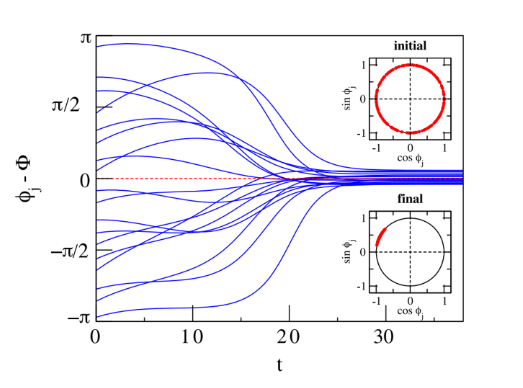
The plot shows the phase difference between individual oscillators (only 18 out of 100 curves are shown) and their average phase $\Phi(t)$. In this case, K is large enough to achieve complete synchronization.

The two smaller plots inside the left figure show the initial state (the 100 oscillators are uniformly distributed on the unit cycle of the complex plane) as well as the final state in which the oscillators are almost perfectly synchronized.

Let us now introduce a synchronization metric that will allow to measure how close N oscillators are to complete synchronization. Recall from calculus that a sinusoidal oscillator with phase $\Phi(t)$ and unit magnitude can be represented in the complex plane as $e^{i \phi(t)}$, where i is the imaginary unit.

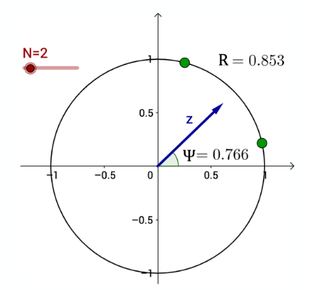
The average of these N complex numbers is another complex number r(t) with magnitude R(t) and phase $\Phi(t)$:

$\large r(t) = R(t) e^{i \Phi(t)} = \frac{1}{N} \sum_{j=1}^N e^{i \Phi_j(t)}$

The magnitude R(t) is referred to as synchronization order parameter. Its extreme values correspond to complete synchronization when R(t)=1 (all oscillators have the same phase) and complete de-coherence when R(t)=0 (that happens when each oscillator has a phase difference $2\pi / N$ from its closest two oscillators).

The visualization at the right shows the unit cycle in the complex plane. Two oscillators are shown as green dots on the unit cycle. The vector z represents the average of the two oscillators. The order parameter in this example is 0.853 (shown as R in this plot), and the phase of z is shown as $\Psi = 0.766$.

Kuramoto Model on a Complete Network¶

The Kuramoto model has been studied in several different variations:

Is the number of oscillators N finite or can we assume that N tends to infinity? (the former is harder to model)
Do the oscillators have the same natural frequency or do their frequencies follow a given statistical distribution? (the latter is harder to model)
Is each oscillator coupled with every other oscillator or do these interactions take place on a given network? (the latter is harder to model)
Is the coupling between oscillators instantaneous or are there coupling delays between oscillators? (the latter is much harder to model)
In the next couple of pages we will review some key results for the asymptotic case of very large N, and without any coupling delays.

Let us start with the simpler case in which each oscillator is coupled with every other oscillator:

$\large \frac{d\phi_i}{dt} = \omega_j + \frac{K}{N} \sum_{j=1}^N \sin(\phi_j - \phi_i)$

The initial phase of each oscillator is randomly distributed in $[0,2\pi)$. The coupling network between oscillators, in this case, can be thought of as a clique with equally weighted edges: each oscillator has the same coupling strength with every other oscillator.

Further, let us assume that the natural angular velocities of the N oscillators follow a unimodal and symmetric distribution around its mean $E[\omega_i] = \Omega$.

When do these N oscillators get synchronized? It all depends on how strong the coupling strength K is relative to the maximum difference of the oscillator natural frequencies.

If K is close to 0 the oscillators will move at their natural frequencies, while if K is large enough, we would expect the oscillators to synchronize.

Intuitively, we may also expect an intermediate state in which K is large enough to keep smaller groups of oscillators synchronized – but not all of them.

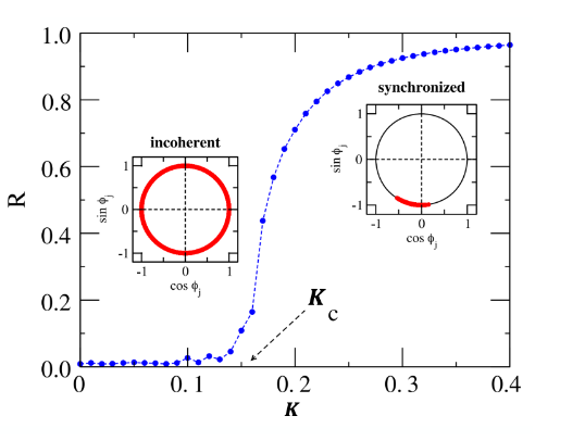
The visualization shows the asymptotic value of the order parameter R(t) (as t tends to infinity), as a function of the coupling strength K.

For smaller values of K, the oscillators remain incoherent (i.e., not synchronized).

As K approaches a critical value $K_c$ (around 0.16 in this case), we observe a phase transition that is referred to as the “onset of synchronization”.

For larger values of $K > K_c$, the order parameter R increases asymptotically towards one, suggesting that the oscillators get completely synchronized.

For the asymptotic case of very large N, Kuramoto showed that as K increases, the system of N oscillators shows a phase transition at a critical threshold $K_c$.

At that threshold, the system moves rapidly from a de-coherent state to a coherent state in which almost all oscillators are synchronized (and so the order parameter R increases rapidly from 0 to 1).

A necessary condition for the onset of complete synchronization is that

$\large K \ge K_c = \frac{2}{\pi \Omega}$

This visualization shows numerical results from simulations with N=100 oscillators in which the average angular frequency is $\Omega = 4$ rads/sec, and $K_c \approx 0.16$.

Kuramoto Model on Complex Networks¶

What happens when the N oscillators are coupled through a complex network? How does the topology of that network affect whether the oscillators get synchronized, and the critical coupling strength?

This problem has received significant attention in the last few years – and there are limited results but only for special cases and only under various assumptions.

First, in the case of an undirected network with adjacency matrix A, the Kuramoto model can be written as follows,

$\large \frac{d\phi_i}{dt} = \omega_j + K \sum_{j=1}^N A_{i,j} \sin(\phi_j - \phi_i)$

A common approximation (referred to as “degree block assumption” – we have also seen it in Lesson-9) is to ignore any degree correlations in the network, and substitute $A_{i,j}$ with its expected value according to the configuration model:

$\large A_{i,j} \approx k_i \frac{k_j}{2m} = \frac{k_i k_j}{N \bar{k}}$
where $\bar{k} = 2m / N $ is the avg node degree and m is the number of edges
- using the approximation karuto model becomes
- $\large \frac{d\phi_i}{dt} = \omega_j + \frac{K}{\bar{k}} \sum_{j=1}^N \frac{k_i k_j}{N } \sin(\phi_j - \phi_i)$
- note that as $N \rightarrow \infty$ the summation remains finite

Under this approximation, a necessary condition for the onset of synchronization is that the coupling strength $\frac{K}{\bar{k}}$ is larger than the following critical threshold:

$K_c = \frac{2}{ \pi \Omega } \frac{\bar{k}}{\bar{k^2}}$
where $\bar{k^2}$ is the second moment

This formula predicts a very interesting result: for power-law networks with degree exponent $2 \lt \gamma \le 3$, the network will always get synchronized, even for a very small K, because the second moment $\bar{k^2}$ diverges.

The visualization shows simulation results of heterogeneous oscillators on power-law networks with degree exponent $\gamma = 3$ (the networks are constructed with the Preferential Attachment model). The natural frequencies of the oscillators vary uniformly in the interval [−1/2,1/2]. The onset of synchronization is not exactly at 0 – but close to 0.05. The small deviation from the theoretically predicted result does not seem to be a consequence of finite N because the critical threshold remains close to 0.05 even as N increases.

We have seen this ratio of the first two moments of the degree distribution several times earlier in the course, including in the friendship paradox, the epidemic threshold, and the critical threshold for random failures. When the second moment diverges, we saw in Lesson-9 that the epidemic threshold goes to 0, and earlier in this Lesson that the critical threshold for random failures goes to 1. Something similar happens here: networks with major hubs get easily synchronized, even with very minor coupling strength.

Adaptive (or Coevolutionary) Networks¶

The most challenging class of problems in network dynamics is related to Adaptive or Coevolutionary networks.

Here, there are two dynamic processes that are coupled in a feedback loop, as shown in this illustration:

The topology of the network changes over time, as a function of the dynamic state of the nodes,
The state of the nodes and/or edges changes over time, as a function of the network topology.

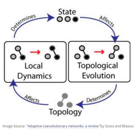
In the illustration, we see a small network of three nodes. Each node can be in one of two states: grey and black. The state of a node depends on the state of its neighbor(s). But also whether two nodes will connect or disconnect depends on their current state.

Adaptive network problems are common in nature, society, and technology. In the context of epidemics, for instance, the state of an individual is dynamic (e.g., Susceptible, Exposed, Infectious, Recovered), depending on the individual’s contacts. That contact network is not static, however – infectious people (hopefully) stay in quarantine, while recovered people may return back to their normal social network.

Closing the feedback loop, such changes in the contact network can also affect who else will get exposed.

Another example of an adaptive network is the brain. The connections between our neurons are not fixed. Instead, they change through both short-term mechanisms (such as Spike-Timing-Dependent Plasticity or STDP) and longer-term mechanisms (such as axon pruning during development), and they affect both the strength of existing connections and the presence of synapses between nearby neurons. Importantly, these synaptic changes are largely driven by the activity of neurons. The Hebbian theory of synaptic plasticity, for instance, is often summarized as “neurons that fire together, wire together” – a more accurate statement would be that if neuron A often contributes to the activation of neuron B, then the synaptic connection from A to B will be strengthened. The connection from A to B may be weakened in the opposite case.

A key question about adaptive networks is whether the two dynamic processes (topology dynamics and node dynamics) operate in similar timescales or not.

In some cases, the topology changes in much slower timescales than the state of the network nodes. Think of a computer network, for instance: routers may become congested in short timescales, depending on the traffic patterns. The physical connectivity of the network however only changes when we add or remove routers and links, and that typically happens in much larger timescales. When this is the case we can apply the “separation of timescales” principle, and study the dynamics of the network nodes assuming that the topology remains fixed during the time period that our model focuses on.

In the more challenging cases, however, the two dynamic processes operate in similar timescales and we cannot simplify the problem assuming that either the topology or the state of the nodes is fixed. We will review a couple of such models in the following pages.

A major question in adaptive network problems is whether the network will, after a sufficient time period, “converge’’ to a particular equilibrium in which the topology and the state of the nodes remain constant. In the language of dynamical systems, these states are referred to as point attractors – and there can be more than one. Other types of attractors are also possible, however. In limit cycles, for instance, the network may keep moving on a periodic trajectory of topologies and node states, without ever converging to a static equilibrium.

Additionally, fixed points in the dynamics of adaptive networks can be stable or unstable. In the latter, small perturbations in the network topology or state of nodes (e.g., removing a link or changing the state of a single node) can move the system from the original fixed point to another.

Consensus Formation in Adaptive Networks¶

In the following, we describe a consensus formation model for adaptive networks that was proposed by Kozma and Barrat. The model is based on the Deffuant model that we studied in Lesson-10.

N agents are endowed with a continuous opinion o(t) that can vary between 0 and 1 and is initially random. Two agents, i and j can communicate with each other if they are connected by a link. Two neighboring agents can communicate if their opinions are close enough, i.e., if $|o(i,t) - o(j,t)| < d$, where d is the tolerance range or threshold.

In this case, the communication tends to bring the opinions even closer, according to the following “update rule”:

$o(i,t+1) = o(i,t) + \mu( o(j,t) - o(i,t) ) $
$o(j,t+1) = o(j,t) + \mu( o(j,t) - o(i,t) ) $
where $\mu \in [0,1/2]$ is a convergence parameter. Consider the case of μ = 1/2 that corresponds to i and j adopting the same intermediate opinion after communication.

The model considers two coexisting dynamical processes: local opinion convergence for agents whose opinions are within the tolerance range, and a rewiring process for agents whose opinions differ more.

The relative frequencies of these two processes is quantified by the parameter $\omega \in [0,1]$.

At each time step t, a node i and one of its neighbors j are chosen at random.

With probability w, an attempt to break the connection between i and j is made: if $|o(i,t) - o(j,t)| > d$, a new node k is chosen at random and the link (i, j) is rewired to (i, k).

With probability 1 − w on the other hand, the opinions evolve according to the previous update rule. if they are within the tolerance range.

If w > 0, the dynamics stop when no link connects nodes with different opinions. This can correspond either to a single connected network in which all agents share the same opinion, or to several clusters representing different opinions.

For w = 0 on the other hand, the dynamics stops when neighboring agents either share the same opinion or differ of more than the tolerance d.

The model is described with the pseudocode shown in Figure (A).

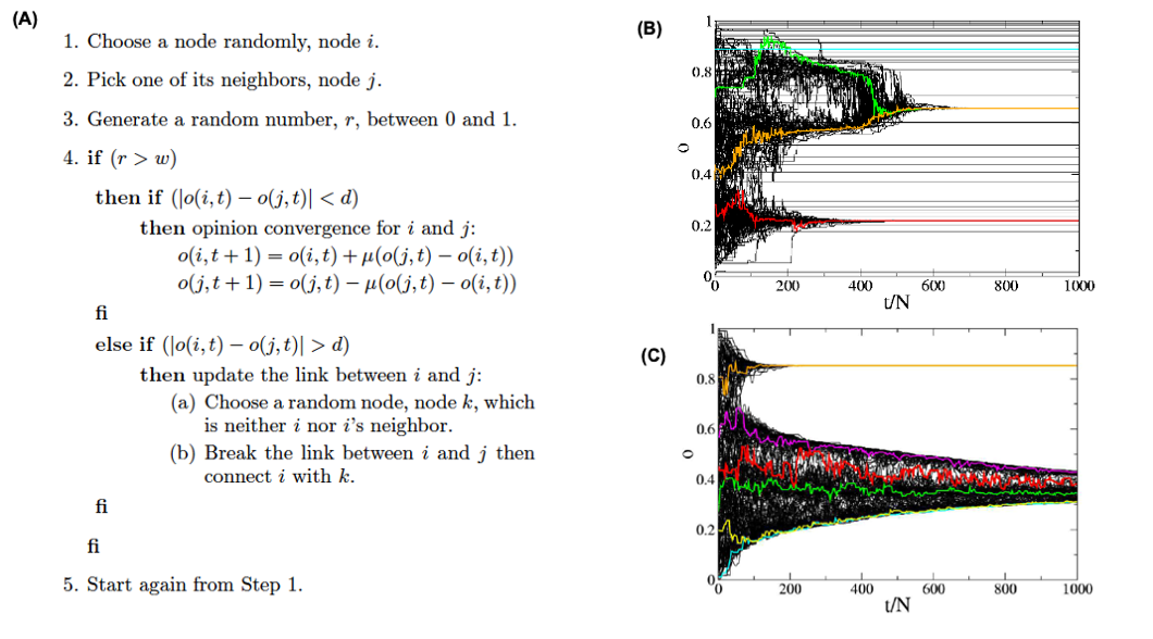
Figures (B) and (C ) show simulation results for N=1000 agents, a tolerance d=0.15, and average node degree $\bar{k}=5$.

Figure (B) refers to the case of a static network without any rewiring, while Figure (C ) refers to the adaptive model we described above (with w=0.7).

The evolution of the opinion of a few individuals is highlighted with color.

When the interaction network is static, local convergence processes take place and lead to a large number of opinion clusters in the final state, with few macroscopic size opinion clusters and many small size groups: agents with similar opinions may be distant on the network and not be able to communicate.

Figure (C), which corresponds to an adaptive network is strikingly in contrast with the static case: no small groups are observed.

The study of Kozma and Barrat showed the following results:

In the case of the static interaction network, two transitions are found: at large tolerance values, a global consensus is reached. For intermediate tolerance values, we see the coexistence of several extensive groups or clusters of agents sharing a common opinion with a large number of small (finite-size) clusters. At very small tolerance values finally, a fragmented state is obtained, with an extensive number of small groups.

In the case of the adaptive interaction network, i.e. when agents can break connections with neighbors with far apart opinions, the situation changes in various ways.

At large tolerance values, the polarization transition is shifted since rewiring makes it easier for a large connected cluster to be broken in various parts. The possibility of network topological change, therefore, renders global consensus more difficult to achieve.

On the other hand, for smaller tolerance values, the number of clusters is drastically reduced since agents can more easily find other agents with whom to reach an agreement. A real polarized phase is thus obtained, and the transition to a fragmented state is even suppressed: extensive clusters are obtained even at very low tolerance.

Coevolutionary Effects in Twitter Retweets¶

Coevolutionary effects have also been observed empirically, on social networks.

Think about Twitter. Consider three users: S (speaker), R (repeater) and L (listener) – see the visualization. Initially, R follows S and L follows R. Suppose that R retweets a post of S. The user L receives that message and it may decide to follow user S. When L starts following S, the network structure changes as a result of an earlier information transfer on the network.

Additionally, this structural change will influence future information transfers because L will be directly receiving the posts of S.

How often does this happen? The study by Antoniades and Dovrolis referenced here analyzed a large volume of Twitter data, searching for the addition of new links from L to S shortly after the retweeting of messages of S from R.

In absolute terms, the probability of such events is low: between $10^{-4}$ to $10^{-3}$ , meaning that only about 1 out of 1000 to 10000 retweets of S lead to the creation of new links from a listener L to S.

Even though these adaptation events are infrequent, they are responsible for about 20% of the new edges on Twitter.

Additional statistical analysis showed that the probability of such network adaptations increases significantly (by a factor of 27) when the reciprocal link, from S to L, already existed.

Another factor that increases the probability (by a factor of 2) that L will follow S is the number of times that L receives messages of S through any repeater R.

Such network adaptation effects have profound effects on information diffusion on social networks such as Twitter because they create “echo chambers” – a positive feedback loop in which a group of initially loosely connected users retweet each other, creating additional links within the group, and thus, making future retweets and new internal links even more likely.

L12 Network Modeling¶

Objectives

Appreciate the value of modeling in the context of network science
Become familiar with some commonly used models such as preferential attachment or stochastic block matrix models
Understand the differences between static vs dynamic models, and stochastic vs optimization-driven models
Understand the value of network modeling through case studies

Why Network Modeling?

lets start with a fundamental question. Why do we need network models? where can we use them in practice. Where to use models instead of the actual data that describe real world network.

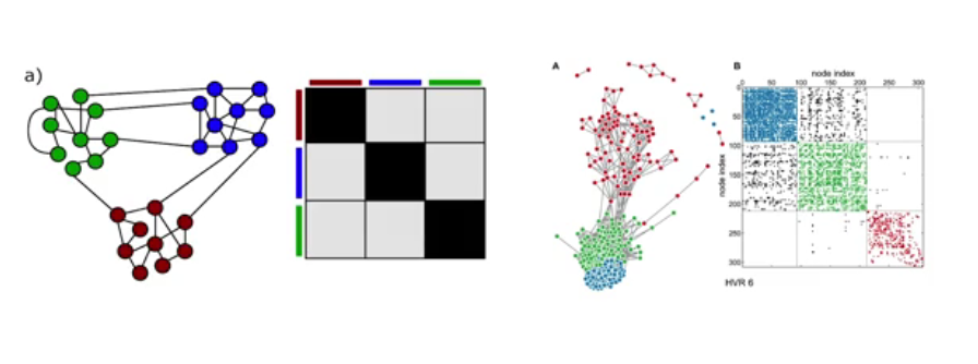
For instance, consider these two networks. The network at the right relates to human malaria parasite which killed some one million people globally every year. We also saw that adjacency matrix of these network ordered so that the existence of the communities (blue green red) are clearly shown. If we want to ask questions about these specific network, we can work with this specific data and not rely any model.

What do we want however, is to ask more general questions about other parasites or larger/smaller instance of this network. The figure at the left shows a network model. It also ahs three communities. This is a stochastic block matrix model and to describe it we need to specify the number of communities, the size and the probability of intra and inter community edges. We can choose these parameters so that these models can product networks that are similar structurally with the malaria network we see at the right. Or we can use the model to create either larger or smaller networks than the malaria network but still with 3 communities. OR we can use this model to generate 100s of network instances, all of them having the size, edge density, same number of communities but different topology.

So, when can we use such an abstract network model instead of the data that specified a given network. A model allows us to describe a given network in a parsimonious manner, with fewer parameters than having to specify the complete adjacency matrix.

Describe a given network in a parsimonious manner, with fewer parameters than having to specify the complete adjacency matrix.
Create an ensemble of many network instances, all of them having the same characteristics.
Examine various network properties and dynamic behaviours if the network was smaller, larger, denser, etc.
when working with noisy data, we can infer whether some of the links in the given network are missing or do not actually exist.
if the model is mechanisitic, it can provide a plausible explanation of how the network came to be in it's current structure.

It also allows us to create an ensemble of many network instances, all of them having the same characteristics. With a model, we can examine various network properties and dynamic behaviors if the network was smaller, larger, denser, etc.

Also, when working with noisy data, we can infer whether some of the links in the given network are missing or they do not actually exists using a model.

Finally if a model is mechanistic, it can provide a plausible explanation on how the network came to be in its current structure. there are also many other reasons to use network models that are often application specific.

Preferential Attachment Model¶

Most real world network show dynamic growth and preferential connections in spite the simple model called the Barabasi Albert model or the preferential attachment. It can generate networks with a power law degree distribution. The model is described as follows:

We start with an initial number of nodes that links between them are chosen arbitrary as long as the node has at least one link. From that point on, the network develops follow two steps at a time.

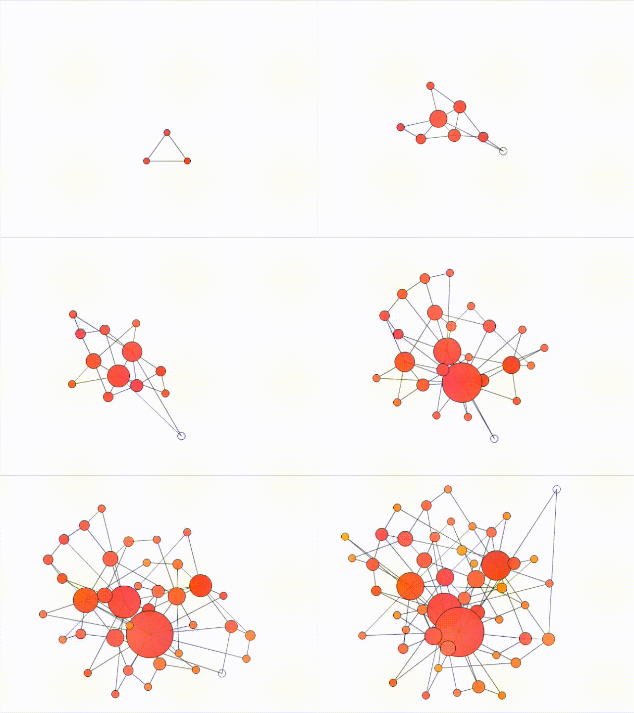
In the growth step, a new node is added with m lengths. In this animation m is equal to two and in the preferential attachment step, the probability that a link of the new node connects to a node i is proportionate to the degree of node i. Preferential attachment is a probabilistic mechanisms. A new node is free to connect any node in the network, whether it is a hub or it has only one link.

The preferential attachment bias however, implies that if a new node has a choice between for example a degree 2 and a degree 4 node, it is twice as likely that the new node will connect to the node of degree 4 rather than the node of degree 2. While most nodes in the network have only few links, a few nodes gradually become hubs. These hubs are a result of rich get richer phenomenon due to preferential attachment. New nodes are more likely to connect to more connected nodes than to the smaller nodes. Hence the larger nodes will acquire links at the expense of the small nodes, eventually becoming hubs.

In the following pages, we will study these models mathematically.

Mathematical Analysis of PA Model¶

Let us now derive mathematically the degree distribution of the Preferential Attachment (PA) model. There are different ways to do these derivations, depending on how rigorous we want to be. Here, we will use the “rate-equation” approach because it is quite general and you can also use it to derive the degree distribution of other growing networks.

Suppose that we add a new node in each time unit, starting from one node at time t=1. So, if N(t) represents the number of nodes at time t, we have that N(t)=t for t >0.

Let $N_k(t)$ denote the number of nodes of degree k at time t. The probability that a node has degree-k at time t is $p_k(t) = \frac{N_k(t)}{N(t)}$ the degree distribution changes with time as we add nodes and edges.

Recall that in the PA model every new node adds m edges to existing nodes. At time t, the total number of edges is $m \times t$ and the sum of all node degrees is twice as large.

The PA model states that the probability $\pi(k)$ that a new node at time t connects to a specific node v that has degree-k is proportional to k:

$\prod(k) = \frac{k}{\sum_j k_j} = \frac{k}{2mt}$

After we add a new node at time t, the average number of edges that are expected to connect to degree-k nodes is:

$m \frac{k}{2mt} N(t) p_k(t) = \frac{k}{2} p_k(t)$

because a new node brings m new edges, and the average number of nodes of degree-k is $N(t)p_k(t)$.

This is also the average number of nodes of degree-k that get a new edge and become nodes of degree-(k+1) – assuming that each node gets at most one new edge.

Similarly, some nodes of degree-(k-1) will get a new edge and they will become nodes of degree-k.

Using the previous expression again, the expected number of such nodes is

$\frac{k-1}{2} p_{k-1}(t)$.

So, considering how many nodes of degree-k we have at time t, how many nodes of degree-(k-1) become nodes of degree-k at time t+1, and how many nodes of degree-k become nodes of degree-(k+1) at time t+1, we can write that the expected number of degree-k nodes at time t+1 as:

$(N+1) p_k(t+1) = N p_k(t) + \frac{k-1}{2} p_{k-1}(t) - \frac{k}{2} p_k(t)$

The previous expression applies to all degrees k>m – but it cannot be used for the minimum possible degree m because there are no nodes with degree m-1 (remember that even a newly born node has m edges).

Instead of having nodes of degree-(m-1) that are “promoted” to nodes of degree-m, we add exactly ONE node of degree-m at each time step.

So the expected number of degree-m nodes at time t+1 is:

$(N+1) p_m(t+1) = N p_m(t) + 1 - \frac{m}{2} p_m(t)$

Note that the previous two expressions give us a recursive process for computing $p_k(t)$ for any value of $k \ge m$ and for any time $t > 0$.

What happens asymptotically, as the network size N increases? It can be shown that the probability distribution $p_k(t)$ becomes stationary, meaning that it does not change with time (we will not prove this step however). We will also see some numerical results that support this claim shortly.

So, instead of $p_k(t)$ we can write that $\lim_{t->\infty} p_k(t) = p_k$.

The expression for nodes of degree- becomes asymptotically

$(N+1) p_m(t+1) - N p_m(t) \rightarrow p_m = 1 - \frac{m}{2} p_m(t)$

Which is equivalent to

$p_m = 1 - \frac{2}{m+2}$

and the expression for nodes of degree-k with k>m becomes asymptotically:

$(N+1) p_k(t+1) - N p_k(t) \rightarrow p_k = \frac{k-1}{2} p_{k-1} - \frac{k}{2} p_k$

Which is equivalent to

$p_k = \frac{k - 1}{k + 2} p_{k-1}$
or
$p_{k+1} = \frac{k}{k + 3} p_k$
when $k \rightarrow k + 1$

We now have a recursive formula that we can easily solve using induction to show that the probability of degree-k nodes is:

$\large p_k = \frac{2m(m+1)}{k(k+1)(k+2)}$ for $k \ge m$

This is the degree distribution equation for the PA model, at least for large networks.

Note that for large degrees (large k), this expression becomes a power-law with exponent 3, i.e., $p_k \approx ck^{-3}$, where c=2m(m+1).

This is the main result of these derivations.

The PA model generates power-law networks – but with a fixed exponent. Further, this exponent is equal to 3, which means that the first moment (mean) of the degree distribution is finite – but any higher moment (including the variance) diverges.

Additionally, note that the degree exponent does not depend on the parameter m. That parameter only controls the minimum degree of the distribution.

Let us now look at some numerical results to get a better insight in the previous results.

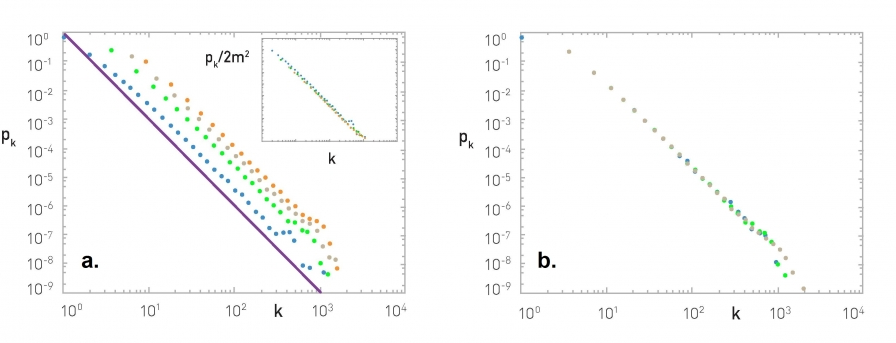
Figure (a) shows what happens as we vary the value of m (blue: m=1, green: m=3, grey: m=5, orange: m=7). The distributions are parallel to each other, having the same exponent. The inset plot shows what happens if we plot $p_k / 2m^2$ – the effect of m disappears, meaning that $p_k$ is proportional to $2m^2$, as also predicted by our earlier mathematical derivation.

Figure (b) shows what happens when we vary the size of the network N (blue: N=50,000, green: N=100,000, grey: N=200,000) – all of the plots have m=3. The resulting degree distributions are practically indistinguishable, supporting our earlier claim that the degree distribution becomes stationary (independent of time) at least for large networks.

Figure (c) shows the degree distribution of the PA network with N=100,000 nodes and m=3. The purple dots are the linearly-binned plot of the empirical degree distribution, while the green dots represent the log-binned version of the same plot. Note that the latter shows more clearly that the degree distribution behaves as a power-law with exponent 3.

Degree Dynamics in PA Model¶

How does the degree of a node change over time in the PA model, as the network grows?

An analytical approach that simplifies the problem considerably is to make two approximations:

ignore the discrete-time increments of the model and use a “continuous-time approximation” instead,
ignore the probabilistic nature of the model and consider a deterministic growth process in which the degree of all nodes increases in a continuous manner based on the PA formula.

Specifically, consider a node i with degree $k_i$ at time t. The rate at which the degree of that node increases at time t is:

$\frac{dk_i}{dt} = m \prod(k_i) = m \frac{k_i}{2mt}$
- which becomes
$\frac{dk_i}{k_i} = \frac{dt}{2t}$
- after integration we get
$\ln k_i = \frac{1}{2} \ln t + c$ which c is constant
- Exponentiating both sides
$k_i = t^{1/2} e^c$

The initial condition is that $k_i(t_i) = m$, where $t_i$ is the time instant that node-i is born.

So, the degree of node i increases with time as follows, for $t > t_i$:

$k_i(t) = m(\frac{t}{t_i})^{1/2}$

This simple derivation predicts a couple of interesting facts:

First, the degree of all nodes is expected to increase with the square-root of time, i.e., sublinearly. The sublinearity is expected because each new node brings the same number of links m but it has to distribute those links to a growing number of nodes.
Second, older nodes (nodes that were added earlier in the model), accumulate a larger degree over time. In fact, the maximum degree is expected to be the degree of the first node added in the network, i.e., $k_{max}(t) \approx \sqrt(t)$. So, the PA model can capture the “first-mover advantage” that is often seen in economy, especially when companies compete for new products or services.

This last point also highlights a shortcoming of the PA model: it cannot capture that different nodes may have different “attractiveness” for new links. The only node feature that matters is the time at which the node is born.

There are several variations of the PA model that introduce additional node parameters (such as a “quality” factor for each node), and/or different network processes (such as removal of existing nodes or edges, or rewiring of existing edges).

The visualization shows numerical results for nodes born at different times (purple for the node born at t=1, orange for the node born at t=100, etc). All curves increase approximately with an exponent of $\beta = 1/2$ (note the log scale of the x and y axes).

Of course there are statistical fluctuations because these numerical results do not use the deterministic approximation of the previous derivations. The green curve represents the function $t^{1/2}$.

The lower plots show the degree distribution at three different snapshots of the growth process.

Nonlinear Preferential Attachment¶

There are many variations of the PA model in the literature. Some of them generate special types of networks (such as directed or bipartite) while others include additional processes such as the removal or rewiring of edges or the aging of nodes.

Here, we present a nonlinear variation of the PA model in which the probability $\pi(k)$ that a new node at time t connects to a specific node v that has degree-k is, not proportional to k, but proportional to:

$\prod(k) = ck^{\alpha}$
where c is a constant to ensure $\sum_k p_k = 1$
and $\alpha$ is a positive exponent that may be larger or smaller than one.

Of course the basic PA model results from $\alpha = 1$.

This nonlinear PA model can be analyzed mathematically using the same methodology we studied earlier (the rate-balance approach) – you can try it yourself or look at the textbook (Advanced Topics 5.C).

If $\alpha < 1$, the bias to connect to higher-degree nodes still exists but it is weaker than in the linear PA model. This changes the degree distribution qualitatively – it becomes the product of the power-law term $k^{-\alpha}$ and an exponential-decay term:

$\large p_k \approx k^{-\alpha} e^{-m_{\alpha} k^{1-\alpha}}$
where $m_{alpha}$ is a constant that depends on $\alpha$ and m (the number of edges that each new node brings). This distribution is referred to as “stretched exponential” – the exponential term dominates for large values of k. The variance of the stretched exponential distribution does not diverge – such networks do not have large hubs and they do not exhibit the extreme properties of power-law networks we have seen in earlier lessons (such as the lack of an epidemic threshold).

Let’s also compare the degree dynamics of this model with the basic PA model we studied in the previous page. Recall that, when $\alpha = 1$, we saw that $k_{max} \approx \sqrt{t}$. When $0 < \alpha < 1$, we can show that $k_{max}$ increases logarithmically: $k_{max} \approx (\ln t)^{1/(1-\alpha)}$

What happens when $\alpha > 1$? Intuitively, the bias to connect to higher-degree nodes comes stronger. The resulting networks have fewer but larger hubs than $\alpha = 1$ – and the vast majority of the nodes connect only to those hubs. If $\alpha$ is sufficiently high all new nodes will connect to the first node because the degree of that node is higher, creating a hub-and-spoke (or “star topology”) network.

The maximum degree, in that case, increases linearly with ”time”, $k_{max} \approx t$, because all new edges connect to the same node.

The previous results are illustrated with numerical results in the visualizations at the top of the page, showing the degree distribution for three values of $\alpha$ (0.5, 1 and 1.5 with N=10,000 nodes) and the maximum degree dynamics for $\alpha= 0.5,1 \text{ and } 2.5$.

Link-Copy Model¶

The PA model is simple (it has only one parameter) and it can generate a power-law degree distribution. However, the exponent of that distribution is fixed (equal to 3) and so the PA model does not give us the flexibility to adjust the exponent of the degree distribution to the same value that a given network has.

Let us now study another simple model that can also generate power-law networks but with any exponent we want. Additionally, this model can be used to create directed or undirected networks (we present it here in the context of directed networks).

The model is probabilistic and it also generates a growing network (one new node at a time) – as in the case of PA. Specifically, every time we add a new node v, it connects (with an outgoing edge) to an existing node as follows:

With probability p, v connects to a randomly chosen existing node u. With probability q=1-p, v connects to a random node w that u connects to. In other words, v “copies” an outgoing edge of u (if u does not have any outgoing edges, v chooses another node. If no node has an outgoing edge, v connects to a random node). The previous model is referred to as “link-copy” process. An equivalent way to describe the model is that, with probability q=1-p, node v selects a random edge in the network, say from a node u to a node w, and v connects to w.

The previous process can be repeated for m>1 new outgoing edges of node v. For simplicity, let us analyze the model for m=1 new edge.

Let us denote as $x_j(t)$ the in-degree of node j at time t. How does $x_j(t)$ increase with time?

There are two cases:

node-j is selected randomly (with probability p) from a new node and it gains one incoming edge. At time t, there are N=t nodes (recall that we add one node at each time unit), and so the probability that a node-j will get a new incoming edge at time t in this manner is p/t.
an incoming edge of node-j is selected with probability q – and node-j gains again one incoming edge. The probability of that happening at time t is $\frac{q_j(t)}{t}$ because node-j has $x_j(t)$ incoming edges at that time.

The following analysis will rely on the same assumptions we used in the PA model, i.e., continuous-time approximation and deterministic degree dynamics.

So, we can write a (deterministic) differential equation that expresses the rate at which node-j gains edges:

$\large \frac{dx_j}{dt} = \frac{p}{t} + \frac{qx_j}{t} = \frac{p + qx_j}{t} $

The initial condition for each node-j is that $x_j(t_j) = 0$, where $t_j$ is the time that j was born.

If we index the nodes based on their time of birth (so that node-1 is born at time t=1, node-2 is born at time t=2, etc), we can write that $x_j(j) = 0$ for all j.

The previous differential equation is easy to solve if we rewrite it as

$\large \frac{dx_j}{p + qx_j} = \frac{dt}{t}$

Ingrating each side yields

$\large \frac{1}{q} \ln(p+qx_j) = \ln t + c$
where c is a constant

Exponentiating both sides yields

$\large p + qx_j = e^{cq} t^q$
hence $\large x_j = \frac{1}{q} ( e^{cq} t^q - p )$

With the init condition $x_j(j) = 0$, we get $e^{cq} = \frac{p}{j^q}$.
So the solution for in-degree dynamics is:

$\large x_j(t) = \frac{p}{q} \left[ (\frac{t}{j})^q - 1 \right] $

After some more math which we will skip we get the following result

the link-copy model creates a power-law degree distribution with exponent:

$\large \frac{1}{q} + 1 = \frac{2-p}{1-p}$

Note that when p approaches 1, the new node connects to random existing nodes and so there is no bias to connect to nodes with higher in-degree. In that case, the previous exponent diverges and the in-degree distribution decays exponentially fast with k.

As p approaches 0, on the other hand, the power-law exponent approaches 2, which means that both the first and second moment of the degree distribution diverge. The network acquires a hub-and-spoke topology in that case, with every new node connecting to the first node.

For intermediate value of p, we can get any desired exponent larger than 2. For example, for p=1/2, we get that the exponent is equal to 3, as in the PA model. This does not mean, however, that the networks generated by the PA model are identical with the networks generated by the link-copy model for p=1/2.

The link-copy model has been used to explain the emergence of power-law networks in directed networks such as the Web, citation networks or gene regulatory networks. In all such networks there are “copy-edge” mechanisms.

For example, when someone creates a new Web page, it is often the case that he/she copies links of other relevant web pages.

Similarly, when writing the bibliography of a research article, authors are often “tempted” to copy references of other relevant articles (hopefully after they have read them!).

And in biology, the process of gene duplication creates multiple copies of the same gene. Those genes have the same promoters, and so, at least initially, they can be regulated by the same transcription factors.

Over time, mutations may change the promoter of a gene, creating regulatory differences in the incoming edges of different gene copies.

Generating Networks with Community Structure¶

In the previous models, our focus has been on the degree distribution. That is an important property of a network – but it is not the only key feature.

As we saw earlier, another common property of many real-world networks is clustering and the presence of communities.

There is no reason to expect that the PA model and its many variants can generate any non-trivial community structure.

In fact we have already seen some models earlier that can generate clustering and/or communities. Recall the Watts-Strogatz model from Lesson-5: it can generate strong clustering (similar to that in regular mesh networks) – but it cannot generate communities and its degree distribution is not a power-law.

Additionally, in Lesson-8 we presented two methods to generate networks with a given community structure: the Girvan-Newman (GN) model and the LFR method. Recall that the latter can generate networks with both a power-law degree distribution and a power-law community size distribution.

Here, we briefly present one more model to construct networks with strong clustering and community structure: the Stochastic Block Model (SBM). The model description is very simple: we are given the number of nodes n, the number of edges m, the number r of communities and their sizes n1,n2,...,nr (with $\sum{i=1}^r n_i = n$), and a symmetric r-by-r probability matrix P.

The (i,j) element of P is the probability that a node of community i connects with a node of community j, i.e., $P(u \leftrightarrow v | u \in i, v \in j)$. The diagonal elements of P represent the probability that nodes of the same community connect to each other – those elements are typically larger than the non-diagonal elements. The rows and columns of P are not probability distributions, hence they do not necessarily sum to one.

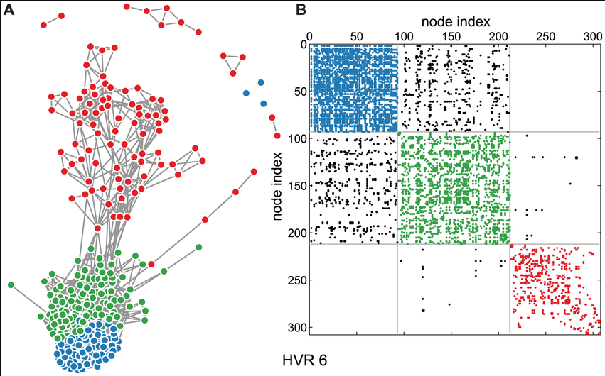
Stochastic block modeling identifies network communities. HVR 6 is shown in two forms, colored according to the best partition into three communities. (A) A force-directed visualization of the network with the identified communities labeled by color. (B) Adjacency matrix in which the ordering of rows and columns has been permuted to match the inferred communities. Diagonal colored blocks are within-community links, and off-diagonal blocks are between-community links. The matrix is shown symmetrically to aid the eye.

Note that SBM models can generate a clearly defined community structure and strong clustering within each community – but it does not control the degree distribution or other network properties. Additionally, the communities are “flat” – without any hierarchical structure.

There is a rich literature, mostly in statistics and machine learning, that focuses on the estimation of the SBM model parameters from network data.

Later in this lesson we will study a more general approach, referred to as Hierarchical Random Graph (HRG) model, and we will present there a statistical approach to estimate the model parameters.

Generating Networks with Degree Correlations¶

Another important network property is the presence of correlations in the degrees of adjacent neighbors. As we have seen in Lesson-3, in assortative networks nodes tend to connect to nodes with similar degree, while in disassortative networks the opposite happens. How can we create networks that exhibit assortative or disassortative behavior?

Suppose that we are given a network (it could be a network that is generated from another model). We can apply the procedure shown in the following visualization:

Select two random links. Let us call the corresponding four end-points (stubs) as (a,b,c,d), ordered based on their degree so that $k_a \ge k_b \ge k_c \ge k_d$.
If we want to create an assortative network, we can rewire the two links so that the two higher-degree nodes connect, adding the edge (a,b) if that edge does not already exist. Also, we connect the two lower-degree nodes, adding the edge (c,d) if that edge does not already exist.
If we want to create a disassortative network, we do the opposite: we connect the highest-degree node (node a) with the lowest-degree node (node d), and node b with node c.

The previous process is applied iteratively until we cannot find pair of edges that can be rewired.

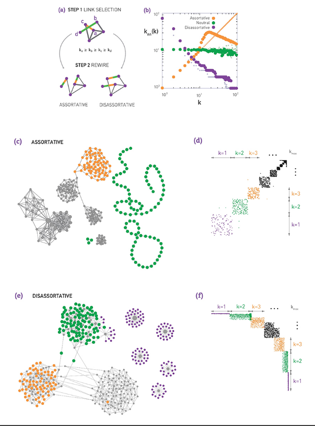
The visualization (b) shows what happens when we apply the previous process on a network generated with the preferential attachment model (with N=1000 nodes, and L=2500 edges). The plot shows the average neighbor node degree $k_nn(k)$ as a function of the degree k (see Lesson-3 if you do not recall such plots). Without applying the previous algorithm, the original network is “neutral”, without any significant degree correlations.

When we apply the previous algorithm to create a disassortative network, the degree correlation between a node and its neighbors become strongly negative (purple points).

On the other hand, when we apply the previous algorithm to create an assortative network, the degree correlations become positive at least up to a certain degree (the reason that the degree correlations become negative for higher degrees is related to the constraint that two nodes can connect with only a single link – the high-degree nodes are few and to maintain a positive degree correlation for high-degree nodes would require several links between the same pair of nodes).

Visualizations (c and d) show an example of an assortative network generated by the previous algorithm and the corresponding adjacency matrix. Note that nodes of degree-1 connect to other nodes of degree-1, while nodes of higher degree connect to other nodes of similarly high degree.

Similarly, visualizations (e and f) show an example of a disassortative network generated by the previous algorithm, and the corresponding adjacency matrix. In this case, nodes of degree-1 connect to the highest degree nodes, while there is also a large number of intermediate-degree nodes that connect to other intermediate-degree nodes.

The previous approach produces maximal assortativity or disassortativity because it keeps rewiring edges to maximize the extent of the degree correlations. Another approach is to apply the previous process probabilistically: with some probability p we perform the previous rewiring step, and with the complementary probability 1-p we leave the two randomly selected edges unchanged. The higher the value of p, the stronger the degree correlations will be.

The following visualization illustrates this process, shows two networks generated in this manner, and it gives average neighbor node degree plots for various values of p.

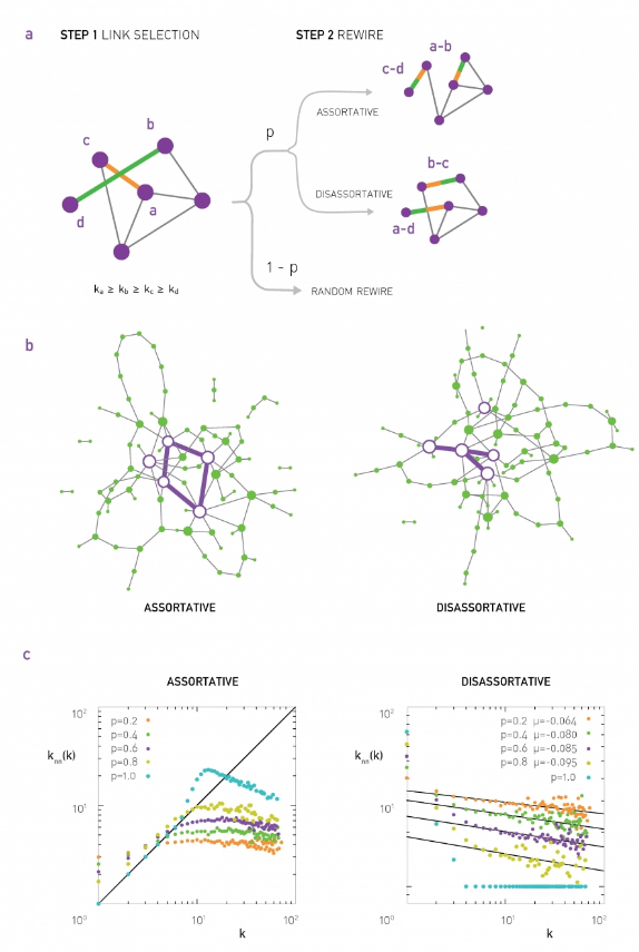
Optimization-based Network Formation Model¶

The models we examined so far are all probabilistic in nature. In practice, and especially in the technological world, networks are not designed randomly. Instead, they are designed to maximize a certain objective function (e.g., minimize cost) subject to one or more constraints. For example, the topology of a computer network may be designed so that it requires few links (routers and their interfaces can be costly) and it offers short paths (and thus small delays).

In social networks, some form of optimization may also be going on “under the surface”. For instance, maintaining a friendship requires time and effort – and so we all (maybe subconsciously) try to have a manageable number of social connections, while at the same time we meet our social need for communication.

Even in biological networks, we may have some underlying optimization through evolutionary mechanisms that gradually select the genotypes with the fittest phenotypes.

So, what happens when a network is designed through an optimization process, without any randomness? What kind of network topologies do we get through that process? We will study here only one such optimization model (out of many different formulations, especially in the literature of communication networks).

Suppose that we design a growing communication network. Nodes arrive one at a time on a given “spatial map”. For simplicity, let us assume that that map is an one-by-one square.

Every new node i connect to one of the existing nodes. If node-i chooses to connect with node-j, the cost of that connection is proportional to $d_{i,j}$, i.e., the Euclidean distance between the two nodes.

This link cost is not our only consideration however. We also want to keep the path length between any pair of nodes short. One way to quantify this objective is the following: Suppose that the very first node represents the “center” of the network – and let $h_j$ be the path length (in number of hops or links) between node-j and the center. If we keep $h_j$ short for all nodes, then the path length between any two nodes will also be short.

Note that because a new node connects to only one existing node, the resulting topology is a tree (and so there is only one path between any two nodes). A tree allows the network to be connected with the minimum number of links (n-1 links for n nodes).

So, on one hand, we want to minimize the cost of the new connection, which is proportional to $d_{i,j}$, and on the other hand, we want to connect to a node j with the smallest possible $h_j$. How can we combine the previous two objectives? Note that they can be conflicting – the node with the smallest $h_j$ may be quite far away from the new node-i.

One approach is to minimize a linear combination of these two metrics. So, when node-i arrives, it connects to the node-j that minimizes the following cost:

$C_j = \delta d_{i,j} + h_j$
where $\delta$ is a model parameter that determines how much weight we give to the cost of the new connection versus the path length objective.

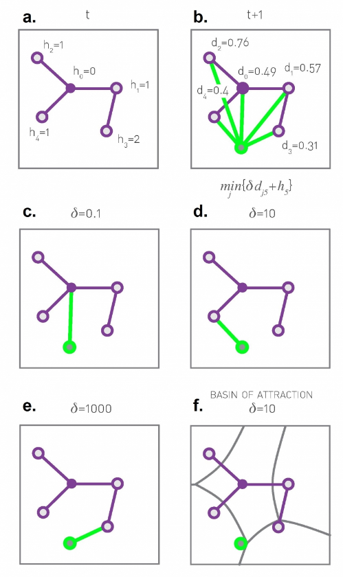
The visualization (a) shows the value of h for the first five nodes in the network. Plot (b) shows the Euclidean distance between the new node (shown in green) and every other node. The plots (c through e) show the optimal selection for node-j for three different values of $\delta$.

If $\delta$ is very low, the new node will prefer to connect directly to the center because the distance-related cost does not matter much.

If $\delta$ is very large, the new node will prefer to connect to the nearest existing node in the unit square.

For intermediate values of $\delta$, both objectives matter and the new node connects with the node that optimizes that trade-off, at least heuristically, based on the nodes that are already in the network.

Plot (f) shows that for a given value of $\delta$, and for each node-j, we can identify a “basin of attraction”, i.e., a region of the unit square in which any new node would decide to connect to node-j.

Now that you have some intuition about this model, think before you move to the next page: what kind of network topology do you expect from this model when $\delta$ is very small? What if $\delta$ is very large? And what may happen for intermediate values of $\delta$?

Optimization-based Network Formation Model (cont’)¶

The previous model (and some variants of it) has been studied extensively. The mathematical analysis of the model is quite lengthy, however, at least for our purposes, and so let us focus on numerical results and some basic insight.

First, what happens when $\delta$ is so low that the distance term does not matter? The maximum possible distance between two nodes in a unit square is $\sqrt{2}$. If $\delta < 1/\sqrt{2}$, we have that $\delta d_{i,j} < 1$. So, for any new node, it is cheaper to connect directly to the center (which has $h_j = 0$) rather than any node with $h_j \ge 1$. In other words, when $\delta < 0.707$, the resulting network has a hub-and-spoke topology because every node connects directly to the center node (see leftmost plots in the visualization – N=10,000 nodes).

On other hand, what happens if $\delta$ is so large that the distance term dominates over the path length $h_j$? When we have N random points on a unit square, the average distance between a point and its nearest neighbor scales with $1/\sqrt{N}$ (do you see why?). The path length to the central node, on the other hand, scales slowly with N (logarithmically with N – recall that the network is a tree). So if $\delta >> \sqrt{N}$, we have that $\delta d_{i,j}$ dominates over the $h_j$ term. In that case, a new node-i will choose to connect to the nearest node-j. The resulting network in this case has an exponential degree distribution, as it is highly unlikely that a node will be the nearest neighbor to many other nodes.

When $\delta$ is between these two extremes ($1/\sqrt{2}$ and $\sqrt{N}$), the model produces topologies with a strong presence of hubs. The hubs connect to many other nearby nodes (i.e., the cost of those connections is quite low) and additionally the few hubs connect either directly to the center node or indirectly, through another hub node, to the center (i.e., the hubs have low $h_j$ value). This hierarchical structure allows almost all nodes in the network to have a very low cost value $C_j$ . The resulting degree distribution can be a power-law – even though the exact shape of the distribution depends on the value of N and 𝛿.

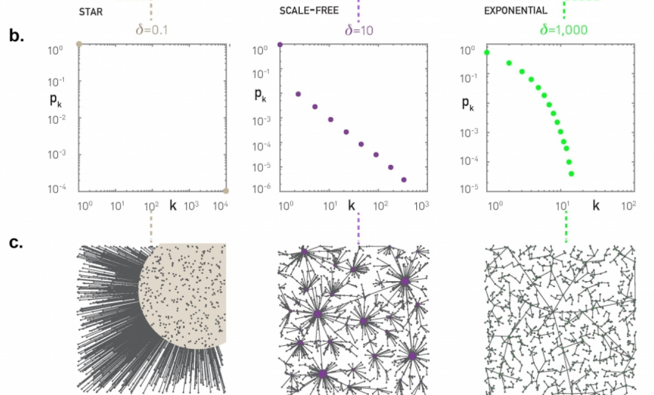
We have seen several models so far that are very different with each other – but they can all create power-law degree distributions. What does this mean?

It is possible that very different mechanisms (e.g., preferential attachment, link-copy, optimization of cost versus path-length, etc) can all create the same network statistics – in terms of the degree distribution or even other properties (clustering, diameter, etc). So we should be careful to not jump into conclusions about the mechanism that has generated a given network, just because that network exhibits a certain statistical property.

Hierarchical Graph Model¶

The previous models are ”stylized” – in the sense that they have only 1-2 parameters and their main goal is to show how a certain network property (e.g., a power-law degree distribution) can be achieved through a simple mechanism (e.g., preferential attachment).

What if we want to create a network model that meets many of the properties of real-world networks, including:

heavy-tailed degree distribution,
strong clustering,
presence of communities, and
hierarchical structure (small and tight communities embedded in larger but looser communities)?

We will now present a model that can meet, to some extent, all these properties. The model is referred to as Hierarchical Random Graph (HRG) and it was proposed by Aaron Clauset and his colleagues.

As opposed to the previous models in this lesson, HRG requires many parameters. Further, these parameters can be calculated algorithmically based on network data, so that the resulting model matches closely the hierarchical density structure of the given network.

First, let us describe the HRG model – without considering the parameter estimation problem. We will examine that problem in the next few pages.

So, suppose we want to create a graph G with n nodes, using the HRG model. The model is described by a dendrogram D, which is a binary tree with n leaves (and so the number of internal nodes in D is n-1).

Each internal node r is associated with a probability $p_r$ – this is the probability that two nodes are connected if r is their lowest common ancestor in D. So, if two graph nodes i and j have the same parent r in D, the two nodes are connected with probability $p_r$.

On the other extreme, if r is the root of D, the probability $p_r$ represents the probability that any node of G at the left subtree of r connects with any node at the right subtree of r.

So, the complete description of the HRG model requires:

The specification of a dendrogram D with n leaves
An (n-1)-dimensional vector of probabilities $p_r$.

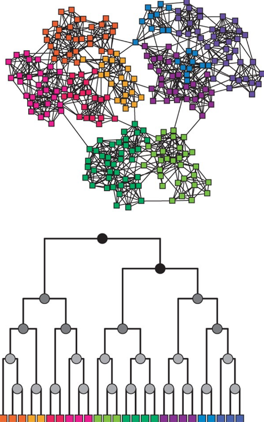
The HRG model is very flexible and it can encompass many different graph models. For instance, if all probabilities $p_r$ are equal to the same value p, we get the G(n,p) model. On the other hand, if we want to create a graph with a strong community structure (as shown in the visualization) we can set $p_r$ to a high value for all internal nodes in D that are lowest common ancestors (LCA) of nodes in the same community.

For example, consider the green community in the visualization – the internal nodes that are LCAs to only green nodes can have a high value of $p_r$ – at least relative to the value of $p_r$ for nodes that are LCAs of nodes that belong to different communities. Similarly for the other communities.

Additionally, if we want to create hierarchical communities, we can have that the lower internal nodes in D have higher values of $p_r$ than the higher nodes in D. This pattern can also generate strong local clustering.

Maximum Likelihood Estimation of HRG Probabilities¶

In the previous page, we assumed that the dendrogram D and the vector $\{p_r\}$ of the HRG model are given. In that case, we can easily create many random graphs G that follow the corresponding HRG model.

What if we do not know these parameters but we are given a (single) network G, and our goal is to statistically estimate the parameters D and $\{p_r\}$ so that the HRG model can produce graphs that are similar to G?

Let us first show how to calculate the probabilities $\{p_r\}$ from a given network G, assuming that the dendrogram D is given (we will remove this assumption at the next page). We will do so using the well-known Maximum Likelihood Estimation (MLE) approach in statistics.

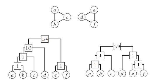
Suppose that r is an internal node in D, and consider all node pairs for which r is the LCA. Let $E_r$ be the number of edges in G that connect those node pairs.

In the left dendrogram of the visualization, the internal node r that is labeled as “1/3” is the LCA of the following node pairs: (a,d), (b,d), (c,d) – and only one of those node pairs is connected (c with d). So $E_r = 1$.

Further, let $L_r$ and $R_r$ be the number of leaves in the left and right subtrees rooted at r.

In the previous example, $L_r = \{a,b,c}$ and $R_r = \{d\}$.

Suppose that someone gives us a vector of probabilities $\{p_r\}$. Recall that the likelihood of a model is the probability that that model will produce the given data. So, the model likelihood is:

$\large \mathcal{L}(D,\{p_r\}) = \prod_{r \in D} p_r^{E_r} (1-p_r)^{L_r R_r - E_r}$
with the convention that $0^0 = 1$

So, if D is fixed, what is the vector $\{p_r\}$ of the HRG model that will result in maximum likelihood?

If we differentiate the previous expression with respect to $p_r$ and set the derivative to zero, we can easily calculate that the optimal value of each $\{p_r\}$ is:

$\large \hat{p_r} = \frac{E_r}{L_r R_r}$
which is simply the fraction of potential edges between the two subtrees of r that actually exist in G.

For these optimal values of $p_r$, we can easily show that the model likelihood is:

$\large \mathcal{L}(D) = \prod_{r \in D} \left[ \hat{p_r}^{\hat{p_r}} (1-\hat{p_r})^{1 - \hat{p_r} L_r R_r} \right]$

It is common to work instead with the logarithm of the likelihood:

$\large log \mathcal{L}(D) = - \sum_{r \in D} L_r R_r h(\hat{p_r})$
where $h(p) = -p log p - (1-p) log(1-p)$.

As an exercise, use this last formula to show that the likelihood of the left dendrogram shown in this visualization is approximately 0.00165. Then, show that the likelihood of the right dendrogram is higher (approximately 0.0433).

How to Find the Optimal Dendrogram?¶

How can we determine the optimal dendrogram D from data?

Unfortunately, it is not possible to derive a closed-form solution for the optimal dendrogram, as we did for the optimal $p_r$ values.

One option would be to construct an iterative search algorithm that samples random dendrograms and tries to find the dendrogram with the highest likelihood $\mathcal{L}(D)$. That may take too long, however, given the super-exponential number of possible dendrograms when n is large (see “food for thought” questions).

It would be much better to sample dendrograms in a biased manner with a probability that is proportional to the likelihood $\mathcal{L}(D)$ – so that dendrograms with higher $\mathcal{L}(D)$ are more likely to be sampled by our search algorithm. We will see how to do so, using a stochastic optimization approach that is known as Markov Chain Monte Carlo (MCMC).

Suppose that an iteration of the algorithm starts with a dendrogram D (e.g., the dendrogram shown at the left of the visualization). We pick an internal node r uniformly at random (other than the root). As shown in the visualization, r identifies three subtrees: the left child-subtree of r (called s), the right child-subtree of r (called t), and the sibling-subtree of r (called u). We can now create two more dendrograms by replacing either s or t with u (as shown in the visualization). Note that these two new dendrograms have preserved the internal relationships in the subtrees s, t and u. We now choose one of the two new dendrograms with equal probability – let us call the new dendrogram D’.

The process we described above describes a Markov Chain, i.e., a probabilistic way to move from one dendrogram to the next, such that only the last dendrogram matters – a Markov Chain does not remember its history.

Now that we have generated the new dendrogram D’, we calculate its likelihood $\mathcal{L}(D')$.

We accept D’ as the new state of the Markov Chain if the likelihood has not decreased (i.e., if $\Delta \mathcal{L} = \mathcal{L}(D') - \mathcal{L}(D) \ge 0 $).

If the likelihood has decreased, we may still accept D’ but we do so with probability

$\large e^{log \Delta \mathcal{L}} = \frac{\mathcal{L}(D')}{\mathcal{L}(D)}$

If we do not accept D’, then we remain with the dendrogram D and pick again a random internal node r.

This process of choosing whether to accept the new state D’ or not is referred to as the Metropolis-Hastings rule.

The interesting property of the previous Markov Chain is that it is ergodic (i.e., we can go from any dendrogram to any other dendrogram with a finite series of the kind of transformation shown in the visualization).

Together with the use of the Metropolis-Hastings rule, this means that the MCMC algorithm presented here ensures that any dendrogram D will be sampled, at least asymptotically, with a probability that is proportional to the likelihood of that dendrogram ${\mathcal{L}(D)}$.

The algorithm terminates when the maximum observed likelihood has reached a “plateau” (meaning that we cannot improve ${\mathcal{L}(D)}$ over a number of iterations).

The previous process is stochastic, and so we may not get the same dendrogram each time we run the algorithm. In practice, however, it has been observed that all resulting dendrograms have roughly the same likelihood.

Hierarchical Graph Model Applications¶

One application of the HRG model is to generate a large ensemble of networks – all of them following the same probabilistic model estimated based on a single given network.

These networks can then be used in simulation studies. For instance, imagine testing a new routing algorithm on many different “Internet topologies” that have been generated from a single snapshot of the current Internet topology.

Another application may be that this ensemble of networks is used as the ”null model” in testing whether a given network follows a certain model or not. For instance, suppose that we have generated an HRG model based on a sample of healthy brain networks – and we have also generated an HRG model based on a sample of brain networks from schizophrenia patients. We can then use these two models to test whether a given brain network belongs in one or the other group.

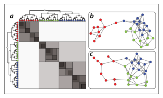
The following visualization shows two different networks (b and c) that were both generated using the HRG model shown at the left (a). The model has 30 nodes. Note that the shading of the internal dendrogram nodes is such that darker means higher probability values. Together with the dendrogram, this visualization also shows the corresponding adjacency matrix, Note that the blue and green communities belong to a larger community that is more loosely connected – and they are less likely to be connected to the red community.

Another application of the HRG model is to detect the presence of false-positive or false-negative edges. This is important in practice because the measured network data is often incorrect or incomplete – especially in the context of biology of neuroscience. So, suppose that we are given a single network $\mathcal{G}$ and we construct an HRG model $\mathcal{G}$ based on $\mathcal{G}$.

If $\mathcal{G}$ predicts that there is a high probability that two nodes X and Y are connected, while these two nodes are not connected in $\mathcal{G}$, we may have a missing edge (false negative) in $\mathcal{G}$.

On the other hand, if $\mathcal{G}$ predicts that there is a low probability that two nodes X and Y are connected, and these two nodes are connected in $\mathcal{G}$, we may have a spurious edge (false positive) in $\mathcal{G}$.

$E[\hat{\tau}] = E\left[\sum_{i \in S}\frac{y_i}{\pi_i}\right] = E\left[\sum_{i \in V}\frac{y_i\, Z_i}{\pi_i}\right] =\sum_{i \in V}\frac{y_i\, E[Z_i]}{\pi_i} = \sum_{i \in V} y_i = \tau $