Localization
Background
How can we determine where we are with a high degree of accuracy? Our robot must be able to sense the world around it.
The idea: Robots are computers at their core. So we can imagine that location is represented as a 1 diminsional line. For our purposes we will take the horizontal y-axis as a measure of probability. At the start of life our robot has no idea where it is so all positions on the line have the same probability. This leads to a state of maximum confusion represented by a uniform distribution. This represents our belief and will be the prior distribution
In order to begin the localization process the world must have some features. Imagine these as identical doors, and our robot must have some sensors to measure the distance to a feature. Upon measurement our initial belief system will be transformed into a series of normal distributions along the location line. This is now our posterior belief.
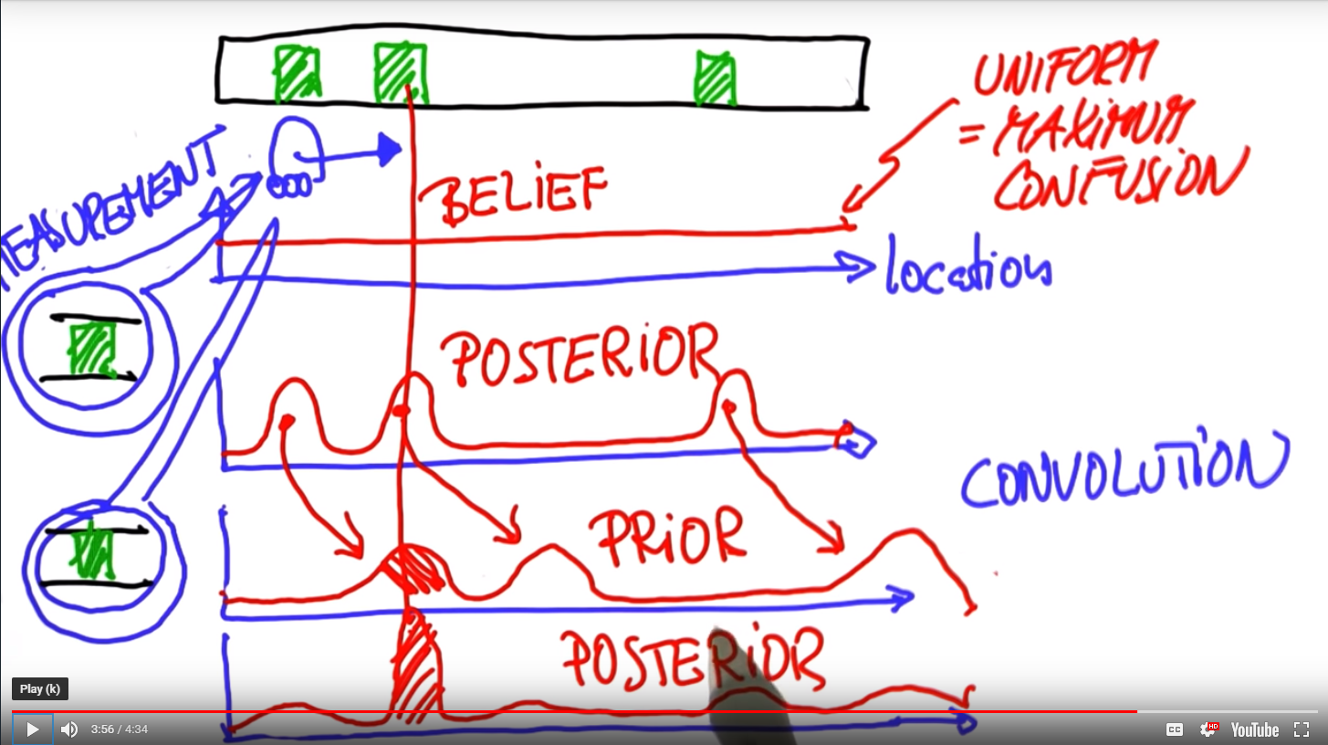
The illustration above better exemplifies what is happening. Notice also what happens when the robot begins to move. The process of moving the beliefs to the right is a convolution. Also note that because robot movement isn't precise the height of the normal bumps is decreasing with each convolution. But in the final posterior there is a spike! This is because the prior distribution illustrates a bump at the same location. Hence the measure of certainty increases at that location.
# imagine a world with 5 cells each with equal probabilty
p=[0.2,0.2,0.2,0.2,0.2]

# Now imagine we need to program a uniform array where the number of cells is changable
p=[]
n=10
################## Put your code here
for i in range(n):
    p.append(1/n)
#####################

print(p)
Let's consider a world made of 5 cells x1 to x5. We've coloured each cell red, or green (x2, x3 are red all others are green). Before turning the robot on we assign each cell an equal probability of being picked, so 0.2 for each cell. At the start our robot is in a state of maximum confusion which is represented by the uniform distribution.
As soon as we turn the robot on it senses the colour red. So we need to incorporate this into our probability distribution. A simple way to do this is to weight the red cells by multiplying. Say we multiply the red cell by 0.6 and the green cells by 0.2
Our new distribution looks like: 0.04, 0.12, 0.12, 0.04, 0.04 (which represents our new belief)
Of course it no longer sums to 1 so we must normalize it ... by 0.36 ( which is the sum of the result)
effectively creating a posterior distribution
# imagine a world with 5 cells each with equal probabilty
p=[0.2,0.2,0.2,0.2,0.2]
# And lets imagine each of these cells is colour coded
t=['green','red','red','green','red']
# And we take a measurement
m = 'green'
# So what is our posterior?
# First we assign some weights
pHit = 0.6
pMiss = 0.2

# We could hard code it ... p[0]=p[0]*pMiss etc etc but that's ugly
# It would be better as a function
def sense(p,Z):
    q=[]
    for i in range(len(p)):
        # Returns a 1(hit) or 0(false)
        hit = (Z == t[i])
        # This will get us the unnormalized values
        q.append( p[i] * (pHit*hit + pMiss*(1-hit) ) )

    # This will normalize
    s = sum(q)
    for j in range(len(q)):
        q[j]=q[j]/s

    return q

# It may not be obvious what's hapenning here but we've effectively incorporated an event
# into our distribution resulting in a normalized posterior
#print(sense(p,m))

# We can call our function multiply times to update/incorporate multiple events
mm = ['green','red']

for k in range(len(mm)):
    p = sense(p,mm[k])

print(p)
Motion-Exact
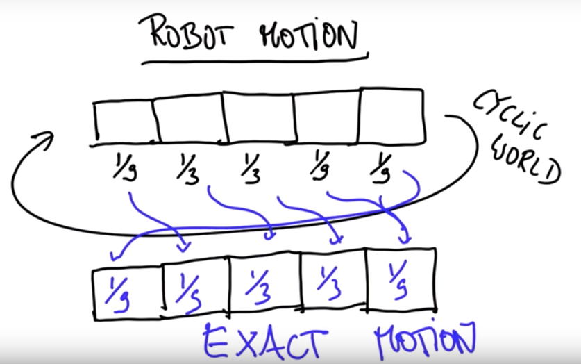
Continuing our grid/cell model from before. Suppose our robot has the following distribution [1/9, 1/3, 1/3, 1/9, 1/9] and wishes to move 1 cell to the right. (We assume that the world is cyclic). We would expect that after moving one cell right our robot has the following posterior distibution [1/9, 1/9, 1/3, 1/3, 1/9]. (We've shifted the probabilities to the right, and cycled the last entry to the start. This is an example of exact motion. Unfortunately robots are not very exact.
Let's program this!
To the above program create a move function that takes an array and shifts the cells one element to the right.
#Program a function that returns a new distribution
#q, shifted to the right by U units. If U=0, q should
#be the same as p.

p=[0, 1, 0, 0, 0]
world=['green', 'red', 'red', 'green', 'green']
measurements = ['red', 'green']
pHit = 0.6
pMiss = 0.2

def sense(p, Z):
    q=[]
    for i in range(len(p)):
        hit = (Z == world[i])
        q.append(p[i] * (hit * pHit + (1-hit) * pMiss))
    s = sum(q)
    for i in range(len(q)):
        q[i] = q[i] / s
    return q

################## Put your code here
def move_v1(p, U):
    q=[]
    for i in range(len(p)):
        q.append(p[(i-U) % len(p)]  )
    return q

def move(p, U):
    # t = len(p)
    # In case U > len(p)
    t = U % len(p)
    # t elem from the end UNION (t-1) elem from the start
    q = p[-t:] + p[:-t]
    return q
#####################################
print(move(p, 2))
Motion-InAccurate
Unfortunately robots are rarely precise in their movements. In general a movement will have a margin of error that must be factored in.
Suppose our robot has a 0.8 chance of an accurate move. 0.1 chance of erring on the short side and 0.1 chance of erring on the long side. For a movement of 1 unit we have 0.1 chance of landing on the same square (not moving at all) and a 0.1 chance of landing 2 squares away, and a 0.8 chance of getting it right, moving exactly 1 square right as expected. How does this impact the posterior distribution? As you might expect the posterior distribution should reflect expected values.
Let's say pinit = [0,1,0,0,0]
Suppose for U=2 we have the following:
$P(X{i+2}|Xi) = 0.8 $
$P(X{i+1}|Xi) = 0.1 $
$P(X{i+3}|X_i) = 0.1 $
then our expected posterior is [0, 0, 0.1, 0.8, 0.1]
In code:
def move(p, U):
    q = []
    for i in range(len(p)):
        s = pExact * p[(i-U) % len(p)]
        s = s + pOvershoot * p[(i-U-1) % len(p)]
        s = s + pUndershoot * p[(i-U+1) % len(p)]
        q.append(s)
    return q
What if we wanted to simulate 1000 moves?
for i in range(1000):
    p = move(p,i)
Should return approx [0.2,0.2,0.2,0.2,0.2]. It won't be this clean though as the decimal places will be greater. What is happening here is convergance to a limiting, or stationary, distribution which in this example is a uniform. Why? Each movement represents a loss of information. The limiting distribution is simply a complete loss. The robot ends up in the same state of maximum confusion it began in.
Summary
The ideas of sense and move represent the basic building blocks of localization. They have a circular relationship. Each time the robot moves it must stop to sense it's surroundings in order to determine it's location. With every move it loses information, with every sense it gains information. Later we will measure information in the distribution (Entropy).
Consider
measurements = ['red', 'green']
motions = [1,1]

for i in range(2):
    p = sense(p,measurements[i])
    p = move(p,motions[i])
Yields:[0.21157894736842103, 0.1515789473684211, 0.08105263157894739, 0.16842105263157897, 0.3873684210526316]. Notice that the 5th element has the highest probability which is interpretable as the location of the robot after 2 cycles of sensing and moving.
Localization Definition
Bayes Rule
Quick Review: $P(X|Z) = \frac{P(Z|X)P(X)}{P(Z)}$
P(X) is the prior
P(Z|X) is the measurement probability
P(X|Z) is the posterior
Total Probability Theorem
let t = time
then $P(X_i^t) = \sum_j P(X_j^{t-1}) P(X_i | X_j)$
The terms on the right is often also called a convolution
Suppose P(H)=0.5 for a fair coin and P(H)=0.1 for a loaded coin
We select a coin with a 50% chance of being fair
We flip it and observe a Heads
What is the probability it is a fair coin?
P(Fair|Heads) = P(Heads|fair)P(Fair) = 0.5 0.5 = 0.25
P(notFair|Heads) = P(Heads|notfair)P(notFair) = 0.1 0.5 = 0.05
P(Heads)=P(H|Fair)+P(H|!Fair) = 0.1 + 0.5 = 0.6
t/f
(0.25+0.05)/0.6 = 0.83
Kalman Filters
Intro - Tracking
Previously we discussed localization, and the problem of dealing with noise from sensors. In this section we discuss tracking. Kalman filters involves a continuous uni-modal view of the environment vs the localization Discrete multimodal view of the universe. Consider a sensor on a car that senses an object at multiple times. Then we should be able to determine the object location at a time in the near future.
Recall the markov model where we divide the world into discrete cells and assign probabilities to compute a histogram like distribution. A Kalman filter uses a gaussian/normal distribution, rather than a uniform, in order to derive it's predictions. Of course we prefer a normal with a small variance, leading to better error margins.
from math import *

def mynorm(mu,sigma2,x):
    const = (1/sqrt(2*pi*sigma2))
    expon = exp( -0.5*(x-mu)**2 / sigma2 )
    result = const*expon
    return result

mynorm(10,4,8) # Note that if you change x to the value of mu you wil get the MLE
Recall
- Measurements require a product, and motion requires a convolution!
- Measurements require Bayes Rule, and motion requires Total Probability
Kalmans Filters oscillate between Measurement and prediction
- Measurements requiring a product using Bayes (similar to before)
- Predictions requiring Total Probability and convolutions
Each measurement will produce a new gaussian which will be used to update the prior. The result being a posterior gaussian whose mean is between the prior and the new measurement. BUT the new variance will be smaller than either the measurement and the prior. Why? because the more info we have the more certain we become, hence less dispersion. Our posterior will be a weighted distribution of the prior and the measurement.
Let P(m1,s1) be our prior and M(m2,s2) be our measurement
Our updated measurement has
- new_mu = (1/(s1+s2))(s2m1+s1*m2)
- new_vr = (1/ ( (1/s1)+(1/s2) ) )
and our prediction function has
- new_mu = (m1+m2)
- new_vr = (s1+s2)
Together they are the basic building blocks of a 1-dim kalman filter
def update(m1,s1,m2,s2):
    new_mu = (1/(s1+s2))*(s2*m1+s1*m2)
    new_vr = (1/ ( (1/s1)+(1/s2) ) )
    return new_mu,new_vr

def predict(m1,s1,m2,s2):
    new_mu = m1+m2
    new_vr = s1+s2
    return new_mu,new_vr

# weightedNorm(10,4,12,4)
# weightedNorm(10,8,13,2)
# Here's a super simple Kalman Filter in one dimension

def update(mean1, var1, mean2, var2):
    new_mean = (var2 * mean1 + var1 * mean2) / (var1 + var2)
    new_var = 1/(1/var1 + 1/var2)
    return [new_mean, new_var]

def predict(mean1, var1, mean2, var2):
    new_mean = (mean1+mean2)
    new_var = (var1+var2)
    return [new_mean, new_var]

measurement = [5., 6., 7., 9., 10.]
motion = [1., 1., 2., 1., 1.]
measurement_sig = 4.
motion_sig = 2.
mu = 0.
sig = 10000.


for i in range(len(measurement)):
    print('start  {}'.format([mu,sig]))
    [mu,sig] = update(mu,sig,measurement[i],measurement_sig)
    print('updat  {}'.format([mu,sig]))
    [mu,sig] = predict(mu,sig,motion[i],motion_sig)
    print('pred   {}'.format([mu,sig]))

print('Final {}'.format([mu,sig]))
Higher Dimensions
This is where things get complicated.
Suppose you are observing a car in 2 dimensional space. At time t=0 you abserve the car at position (x1,y1). You continue to observe the car at 2 more time points. Then you can make a reasonably good prediction of the location at time t=3 based on the previous locations as well as the velocity.
This time around we start with a multivariate gaussian with a mu vector as the mean and a covariance matrix as the variance. We also must another factor into our calculations namely velocity denoted $\dot{x}$ note the little dot on top. The result is that in every time step we need to update our location based on initial location as well as velocity. So the movement is in 2 dimensions. This can be difficult to visualize so consider the following illustration.
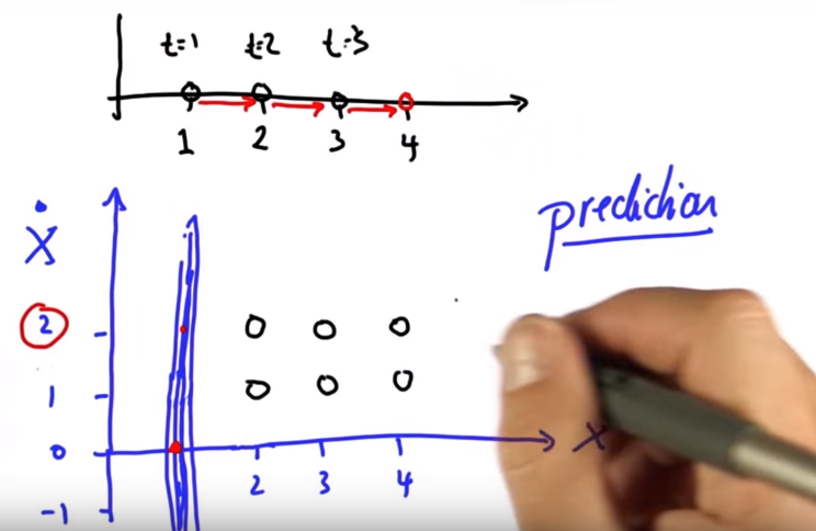
Our initial state is at 1 on the x-axis. The lines you see there are the 3-dimensional gaussian countour viewed from one side. The velocity is given as 2 (vertical axis). The prediction at t=2 is (3,2) The velocity remains unchanged after one step but the location does. Note that time is represented at the top. It's not represented in the lower graph.
When we put these all together we begin to see multiple gaussians.
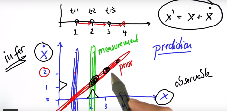
The blue line is the gaussian corresponding with the location measurement at t=1. Similarly for the green line. The red gaussian is the blue tilted (which is the prior). As you can see this can get pretty confusing so we turn to linear algebra to simplify things.
In the above picture we assume a time step of 1 and hence the new state is given as $x' = x + \dot{x}$. However a more general form is $x' = x + \dot{x}*\triangledown t$.
We now begin to formulate the matrices to use in our equations
First we design F to express out state transition. Note what happens when you multiply F with the measurement. the velocity is added to the location to get a new location. But the new velocity remains unchanged.
$
\begin{pmatrix} x' \\ \dot{x'} \end{pmatrix}
\longleftarrow
\begin{pmatrix} 1 & 1 \\ 0 & 1 \end{pmatrix}
\begin{pmatrix} x \\ \dot{x} \end{pmatrix}
$
Similarly we construct an H matrix representing the observation model
$ Z \longleftarrow
\begin{pmatrix} 1 & 0 \end{pmatrix}
\begin{pmatrix} x \\ \dot{x} \end{pmatrix}
$
In more mathematical terms
Define
x = estimate
P = uncertainty covariance
F = state transition matrix
u = motion vector
Z = measurement
H = measurement function
Then prediction is given by
$x' = Fx + u$
$P' = FPF^T$
And the measurement update is given by
$y=z-Hx$
$S = HPH^T$
$K = P(H^T)S^{-1}$ Often called the Kalman Gain
$x' = x + (Ky)$
$P' = (I - KH)P$
%run CS7638/Kalman01.py


# measurements = [[1., 4.], [6., 0.], [11., -4.], [16., -8.]]
# initial_xy = [-4., 8.]

# measurements = [[1., 17.], [1., 15.], [1., 13.], [1., 11.]]
# initial_xy = [1., 19.]
measurements = [[5., 10.], [6., 8.], [7., 6.], [8., 4.], [9., 2.], [10., 0.]]
initial_xy = [4., 12.]

dt = 0.1
x = matrix([[initial_xy[0]], [initial_xy[1]], [0.], [0.]]) # initial state (location and velocity)
u = matrix([[0.], [0.], [0.], [0.]]) # external motion

#### DO NOT MODIFY ANYTHING ABOVE HERE ####
#### fill this in, remember to use the matrix() function!: ####

# initial uncertainty: 0 for positions x and y, 1000 for the two velocities
P = matrix([[0, 0, 0, 0], [0, 0, 0, 0], [0, 0, 1000, 0], [0, 0, 0, 1000]])
# next state function: generalize the 2d version to 4d
F = matrix([[1, 0, dt, 0], [0, 1, 0, dt], [0, 0, 1, 0], [0, 0, 0, 1]])
# measurement function: reflect the fact that we observe x and y but not the two velocities
H = matrix([[1, 0, 0, 0], [0, 1, 0, 0]])
# measurement uncertainty: use 2x2 matrix with 0.1 as main diagonal
R = matrix([[0.1, 0], [0, 0.1]])
I =  matrix([[1, 0, 0, 0], [0, 1, 0, 0], [0, 0, 1, 0], [0, 0, 0, 1]])

###### DO NOT MODIFY ANYTHING HERE #######

def kalman_filter(x, P):
    for n in range(len(measurements)):

        # measurement update
        print("------HOORAY-Measurement-----")
        print('x0={}'.format(x))
        x = (F * x) + u
        P = F * P * F.transpose()
        print('x1={}'.format(x))

        # prediction
        #print("------HOORAY-Prediction------")
        Z = matrix([measurements[n]])
        print('Z={}'.format(Z))
        print(Z)
        y = Z.transpose() - (H * x)
        S = H * P * H.transpose() + R
        K = P * H.transpose() * S.inverse()
        x = x + (K * y)

        P = (I - (K * H)) * P

    return x,P

kalman_filter(x, P)
Particle Filters
Intro
Easiest to program and one of the strongest methods for estimating the state space.
Recall
| Filter | State space | Belief | Complexity | Robotics |
| Histogram | Discrete | Multimodal | Exponential | Approx |
| Kalman | Continous | Unimodal | Quadratic | Approx |
| Particle | Continous | multimodal | ?? | approx |
At a high level particle filters work by condensing particles in the location corresponding to the highest probabilities.
Consider
%run CS7638/MovingRobot.py

myrobot = robot()

# When used this will cause each execution to be different
# myrobot.set_noise(5.0,0.1,5.0)

myrobot.set(30,50,pi/2)
myrobot = myrobot.move(-pi/2,15)
print(myrobot.sense())

myrobot = myrobot.move(-pi/2,10)
print(myrobot.sense())
The above code is a demonstration of just one particle. In practice though we would use many
N = 1000
p = []
for i in range(N):
    x = robot()
    x.set_noise(0.05, 0.05, 5.0 )
    p.append(x)
Each of these particles/robots can/will move in it's own direction.
p2 = []
for i in range(N):
    p2.append(p[i].move(0.1,5.0))
p = p2
What we need to do now is figure out a way to assign importance weights to them.
w = []
for i in range(N):
    # Z is the result of the sense measurement
    w.append(p[i].measurement_prob(Z))
Now we need to normalize the weights ie $\alpha_i = \frac{w_i}{\sum w_i}$ Now draw from the alphas using resampling methodology and determine their associated particle.
Consider the following weights 0.6,1.2,2.4,0.6,1.2 if summed gets you 6
So we compute our alphas as a1 = 0.6/6 = 0.1 and repeat for the others
Each alpha has a probability of not being sampled and this is key to this filter.
Ex
p3 has a (1-0.4)^5 (0.077) probability of not being sampled
p1 has a (1-0.9)^5 (0.077) probability of not being sampled
the following piece of code implements a resampling wheel. Each weight is represented as a slice of a wheel.
p3 = []
index = int(random.random() * N)
beta = 0.0
mw = max(w)
for i in range(N):
    beta += random.random() * 2.0 * mw
    while w[index] < beta:
        beta = beta - w[index]
        index = index + 1

    p3.append(p[index])
Up until now orientation doesn't matter. However if you repeat the above steps for multiple movements you'll notice that they will converge.
Quiz
# 4 possible states a,b,c,d, and we have n=particles
# Q1 for n=1 What is the probability of 0 particles in state a
# ie - Pr(a=0,n=1) - combinatorics
print(3/4) #=> Pr(b=1,n=1) + Pr(c=1,n=1) + Pr(d=1,n=1)
# Q2 - Pr(a=0,n=4)
print((3/4)**4)
# Q3 - Pr(a=0,n=10)
print((3/4)**10)
# 4 possible states with particles as follows
# a(5particles),b(3),c(3),d(1)    12 Particles in total
# [ 5  3 ] (a,b)
# [ 3  1 ] (c,d)
# 50% move horizontally, and 50% move vertically
# None move diagonally, none stay in the same cell
# After 1 step
print('Step 1')
print('a={}  b={}'.format((0.5*3+0.5*3),(0.5*5+0.5*1)))
print('c={}  d={}'.format((0.5*5+0.5*1),(0.5*3+0.5*3)))

print('Step 2')
print('a={}  b={}'.format((0.5*3+0.5*3),(0.5*3+0.5*3)))
print('c={}  d={}'.format((0.5*3+0.5*3),(0.5*3+0.5*3)))

print('Step Infinity??')
Q3
Suppose you run a particle filter with n=1 particles What will happen?
- It will ignore measurements Yes Because measurements set the weighting factors so it will be resampled
- It will likely fail because it ignores the measurement
- it will NOT ignore motion though, it will still move
Q4 Movement
Consider the following simplistic robot:
We have a simple box car, located at (y,x) NOT (x,y), and our car has a heading of theta.
So we can describe our initial state as (x,y,$\theta$)
Our car also has a steering angle $\alpha$ and a length given by L And we wish to go distance given as d
Notes
- turning angle is relative to the distance(d) divided by the length(L) and multiplied by the steering angle alpha
- the turning radius is relative to the distance divided by the turning angle
- Think of cx,cy as a pivot point, or an observation point
Note that the difference between the 2 primed equations hinges on beta. if beta < 0.001 then turning radius goes to infinity due to division by zero so we must drop the turning radius in our primed equations
Illustrated are the required equations
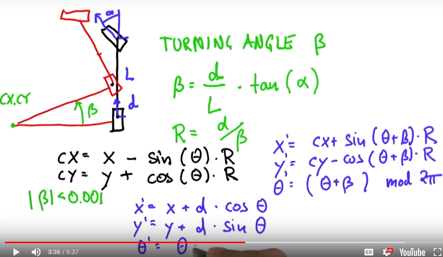
The code can be found here: CS7638_AI4R/L9Q3_ParticleMovement.py Note that it is in Python 2.7? and needs some cleaning to run on python 3
Q5 Sensing
Now we need to implement a sensing(measurement) function. What we do here is measure our bearing to possible landmarks. atan2() returns the orientation of the vector in global co-ordinates and then we adjust for our orientation in the robots local co-ordinates. Mathematically: $atan2(\Delta y, \Delta x) - \theta$ where $\theta$ is the orientation.
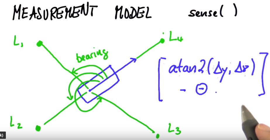
Here's the implementation in Python 2.7 (CS7638_AI4R/L9Q5_ParticleSensing.py)
A full implementation can be found (CS7638_AI4R/L9PS3_FullParticleFilter.py)
5 Searching
Motion Planning
How does a robot plan it's next steps towards it's goal. Planning problem: given a map, a start, end, and a cost function how do we find the minimum cost. To motivate this discussion assume the world is divided into a grid. Where there are two possible actions, move and turn, with the same cost of 1 unit.
First Search Given a grid of available position: first search for all available options/spots and assign a cost. In the code below we begin at (0,0) in the grid and can move left, right, up, or down. Clearly given our current state we can move to (0,1) or (1,0). Both have the same cost: 1, which we will call the g-value. We could choose either for our optimal path.
Assume we choose (0,1) = (col,row)
then our next possible options are (0,2) and (1,1). Again both have a cost of 1
We repeat this process always expanding onto nodes not yet visited
First Search
grid = [[0, 0, 1, 0, 0, 0],
        [0, 0, 1, 0, 0, 0],
        [0, 0, 1, 0, 1, 0],
        [0, 0, 1, 0, 1, 0],
        [0, 0, 0, 0, 1, 0]]

init = [len(grid)-1, len(grid[0])-1]
goal = [0, 0]
cost = 1

delta = [[-1, 0], # go up
         [ 0,-1], # go left
         [ 1, 0], # go down
         [ 0, 1]] # go right

delta_name = ['n', 'w', 's', 'e']

# We implement the logic
def search():

    closed = [[0 for col in range(len(grid[0]))] for row in range(len(grid))]
    closed[init[0]][init[1]] = 1
    expand = [[-1 for col in range(len(grid[0]))] for row in range(len(grid))]
    action = [[-1 for col in range(len(grid[0]))] for row in range(len(grid))]

    g,x,y = 0,init[0],init[1]

    open = [[g,x,y]]

    found = False
    resign = False
    count = 0

    while found is False and resign is False:
        # Check to see if there are unvisited spots
        # print(len(open))
        if len(open) == 0:
            resign = True
            print("I have failed")
        else:
            open.sort()
            open.reverse()
            # This will be the one with the smallest g-value
            next = open.pop()
            #print('choice {}'.format(next))
            g,x,y=next[0],next[1],next[2]
            expand[x][y] = count
            count += 1

            # Did we get to the goal?
            if x == goal[0] and y == goal[1]:
                found = True
                print("Success")
            else:
                for i in range(len(delta)):
                    x2 = x + delta[i][0]
                    y2 = y + delta[i][1]
                    if x2 >= 0 and x2 < len(grid) and y2 >= 0 and y2 < len(grid[0]):
                        if closed[x2][y2] == 0 and grid[x2][y2] == 0:
                            g2 = g + cost
                            open.append([g2,x2,y2])
                            #print([g2,x2,y2])
                            closed[x2][y2] = 1
                            action[x2][y2] = i

    policy = [[' ' for col in range(len(grid[0]))] for row in range(len(grid))]
    x,y = goal[0],goal[1]
    policy[x][y] = '*'

    print('ACTIONS')
    for i in range(len(action)):
        print(action[i])

    while x!= init[0] or y != init[1]:
        x2 = x - delta[action[x][y]][0]
        y2 = y - delta[action[x][y]][1]
        policy[x2][y2] = delta_name[action[x][y]]
        x = x2
        y = y2

    print('POLICY')
    for i in range(len(policy)):
        print(policy[i])

    return action

mvs = search()
#for i in range(len(mvs)): print(mvs[i])
A* Search
Builds upon the first search algorithm. In this case we add a heuristic matrix with the same dimensions as the initial grid, but in the heuristic matrix the elements are less than, or equal, to the distance to the goal. It doesn't necassarily need to be accurate since that would require a path solution. It can be modified or fitted for performance and behaviour. The values in the heuristic matrix are used to minimize the cost of expansion in the first search. It's a guided search of sorts.
NB A heurisitic element should be less than or equal to the distance to the goal
If this doesn't hold than the optimal path may not hold.
# User Instructions:
#
# Modify the the search function so that it becomes
# an A* search algorithm as defined in the previous
# lectures.
#
# Your function should return the expanded grid
# which shows, for each element, the count when
# it was expanded or -1 if the element was never expanded.
#
# If there is no path from init to goal,
# the function should return the string 'fail'
# ----------

grid = [[0, 1, 0, 0, 0, 0],
        [0, 1, 0, 0, 0, 0],
        [0, 1, 0, 0, 0, 0],
        [0, 1, 0, 0, 0, 0],
        [0, 0, 0, 0, 1, 0]]
heuristic = [[9, 8, 7, 6, 5, 4],
             [8, 7, 6, 5, 4, 3],
             [7, 6, 5, 4, 3, 2],
             [6, 5, 4, 3, 2, 1],
             [5, 4, 3, 2, 1, 0]]

init = [0, 0]
goal = [len(grid)-1, len(grid[0])-1]
cost = 1

delta = [[-1, 0 ], # go up
         [ 0, -1], # go left
         [ 1, 0 ], # go down
         [ 0, 1 ]] # go right

delta_name = ['^', '<', 'v', '>']

def search(grid,init,goal,cost,heuristic):
    # ----------------------------------------
    # modify the code below
    # ----------------------------------------
    closed = [[0 for col in range(len(grid[0]))] for row in range(len(grid))]
    closed[init[0]][init[1]] = 1

    expand = [[-1 for col in range(len(grid[0]))] for row in range(len(grid))]
    action = [[-1 for col in range(len(grid[0]))] for row in range(len(grid))]

    x = init[0]
    y = init[1]
    g = 0
    h = heuristic[x][y]
    f = g + h
    open = [[f, g, h, x, y]]

    found = False  # flag that is set when search is complete
    resign = False # flag set if we can't find expand
    count = 0

    while not found and not resign:
        if len(open) == 0:
            resign = True
            return "Fail"
        else:
            open.sort()
            open.reverse()
            next = open.pop()
            f,g,x,y = next[0],next[1],next[3],next[4]
            expand[x][y] = count
            count += 1

            if x == goal[0] and y == goal[1]:
                found = True
            else:
                for i in range(len(delta)):
                    x2 = x + delta[i][0]
                    y2 = y + delta[i][1]
                    if x2 >= 0 and x2 < len(grid) and y2 >=0 and y2 < len(grid[0]):
                        if closed[x2][y2] == 0 and grid[x2][y2] == 0:
                            g2 = g + cost
                            h2 = heuristic[x2][y2]
                            f2 = g2 + h2
                            open.append([f2, g2, h2, x2, y2])
                            closed[x2][y2] = 1

    return expand

mvs = search(grid,init,goal,cost,heuristic)
for i in range(len(mvs)):
    print(mvs[i])
Dynamic programming
Imagine your a robot car. You want to turn left at the coming light but the cars in the left lane refuse to let you in. so you end up missing your turn. Now you need a new plan. How to get to your goal from an unplanned location?
Dynamic planning will create a gradient like grid. ie for each grid cell there is an direction that you need to move in Here's an example ( the 1s represent a wall, G is our goal )
[[V, 1, >, >, >, V],
 [V, 1, >, >, >, V],
 [V, 1, >, >, >, V],
 [V, 1, >, >, >, V],
 [V, >, >, >, 1, G]]
What this is is a set of preprogrammed directions. should the robot find itself in any cell it knows exactly which direction to go.
How we implement this is to apply a value function to the grid. to each cell in the grid it assigns the length of the shortest path to the goal. this is done by recursively taking the min value of it's neighbours plus one
$f(x,y) = min_{x',y'}f(x',y')+1$
Here's an example of how to compute a value grid
grid = [[0, 0, 1, 0, 0, 0],
        [0, 0, 1, 0, 0, 0],
        [0, 0, 1, 0, 0, 0],
        [0, 0, 0, 0, 1, 0],
        [0, 0, 1, 1, 1, 0],
        [0, 0, 0, 0, 1, 0]]

init = [0, 0]
goal = [len(grid)-1, len(grid[0])-1]

delta = [[-1, 0 ], # go up
         [ 0, -1], # go left
         [ 1, 0 ], # go down
         [ 0, 1 ]] # go right

delta_name = ['^', '<', 'v', '>']
cost = 1

value  = [[99 for col in range(len(grid[0]))] for row in range(len(grid))]
policy = [[' ' for col in range(len(grid[0]))] for row in range(len(grid))]

change = True

while change:
    change = False

    for x in range(len(grid)):
        for y in range(len(grid[0])):
            # print(x,y)
            # Sets the goal equal to 0
            if goal[0]==x and goal[1]==y:
                if value[x][y] > 0:
                    value[x][y] = 0
                    change = True
                    policy[x][y] = '*'
                    #print('I was hit')
            elif grid[x][y] == 0:
                for a in range(len(delta)):
                    x2 = x + delta[a][0]
                    y2 = y + delta[a][1]
                    #print(x2,y2,(grid[x2][y2]),(x2 < len(grid)))
                    # check if in bounds
                    if ( x2 >=0 and x2 < len(grid) and y2 >=0 and y2 < len(grid[0])
                        and grid[x2][y2] == 0
                       ):
                        v2 = value[x2][y2]+cost
                        #print(v2)
                        if v2 < value[x][y]:
                            value[x][y]=v2
                            policy[x][y] = delta_name[a]
                            change = True


# The value function
for i in range(len(value)):
    print(value[i])

for i in range(len(policy)):
    print(policy[i])
PID Controls
Topics
- Generating Smooth paths
- Control using PIDs
Previously, we looked at a discrete world composed of a grid. Now we move on towards a more continuous state. The world is still discrete, but we can move in fractions
to smooth our path we
- $y_i=x_i$
- Optimize $(x_i-y_i)^2 + \alpha (y_i-y_{i+1})^2$ where alpha is the data weighting term
To optimize we use gradient descent. The final equation is as follows
$y'_i = y_i - \beta ( y_{i+1} + y_{i-1} - 2y_i )$
Where y' is the new path y and $y_i$ is the old, before smoothing is applied
And $\beta$ is our smoothing weight
PID Control
Suppose we have a car with a fixed velocity. We can alter the steering however. We define the Cross Track Error as the difference between the current location and the intended trajectory. Ideally, we want to be on the intended trajectory. To get there, while moving forward, means we will use the changing CTE to adjust our heading.
If we adjust proportionally to the CTE only, we will end up overshooting, and oscillating. To remedy the oscillation we add another term proprotional to the change in the CTE. Change in CTE is measured from the last 2 cross track errors.
- P for proprotional
- I for integral
- D for Derivative
Systematic Bias Is when your starting point is erroneous. Then your robot will constantly be trying to adjust but because of the bias it will never get there. To visualize this consider a car whose steering is naturally off due to some mechanical error. Maybe it veers right. To this car a straight command would cause veering to the right which must be compensated for. This type of error is remdeied by adding an integral term I
Mathematically:
$\alpha = -\tau_P CTE -\tau_D \frac{d}{dt} CTE -\tau \sum CTE $
steering = -tau_p * CTE - tau_d * diff_CTE - tau_i * int_CTE
In both equations tau is simply a weighting factor. Each term gets it's own tau.
Here is a small snippet pulled from Github. This update comes from a class whose variables are set at initiallization. There are no other functions.
https://github.com/korfuri/PIDController
def Update(self, error, current_time=None):
    if current_time is None:
        current_time = time.time()
    dt = current_time - self.previous_time
    if dt <= 0.0:
        return 0
    de = error - self.previous_error

    self.Cp = error
    self.Ci += error * dt
    self.Cd = de / dt

    self.previous_time = current_time
    self.previous_error = error

    return ((self.Kp * self.Cp)    # proportional term
            + (self.Ki * self.Ci)  # integral term
            + (self.Kd * self.Cd)  # derivative term
    )
Twiddle
A way to try out multiple weightings that reduce the error.
In the example below A(p) would be a call to your PID controller, that returns an error. Generally a cross track error.
# Choose an initialization parameter vector
p = [0, 0, 0]
# Define potential changes
dp = [1, 1, 1]
# Calculate the error
best_err = A(p)

threshold = 0.001

while sum(dp) > threshold:
    for i in range(len(p)):
        p[i] += dp[i]
        err = A(p)

        if err < best_err:  # There was some improvement
           best_err = err
           dp[i] *= 1.1
        else:  # There was no improvement
           p[i] -= 2*dp[i]  # Go into the other direction
           err = A(p)

           if err < best_err:  # There was an improvement
              best_err = err
              dp[i] *= 1.05
           else  # There was no improvement
              p[i] += dp[i]
              # As there was no improvement, the step size in either
              # direction, the step size might simply be too big.
              dp[i] *= 0.95
SLAM
If we leave a robot in an unknown location, in an unknown environment can the robot make a satisfactory map while simultaneously being able to find its pose in that map?
Putting it all together. Using filters to localize and track an object, Search and Planning algo's to plot the movements of the robot, and PID to perform the move.
Our motivating example today will be a robot that moves through a maze (represented by a matrix). It needs to plan it's path, move forward while avoiding collision,
Suppose we require our robot to move from $P_1=(x_1,y_1)$ to $P_2=(x_2,y_2)$. Let the robot's actual position be given as $P=(x,y)$ and let $\theta$ be the heading.
Then $Rx = x-x_1$ and $Ry = y-y_1$ is the current errors
and $dx = (x_2-x_1)$ and $dy = (y_2-y_1)$ is the current change
The current crosstrack error is given as
$CTE = \frac{Ry*dx - Rx*dy}{ \sqrt{dx^2 + dy^2}} $
We also create a variable u to help us know when to move to the next segment of our map, the move from P2 to P3.
ie we increment our segment when
$u= \frac{Rx*dx + Ry*dy}{ dx^2 + dy^2} > 1$
Below we can see an example of a basic, but complete, working robot
%run CS7638/SLAM_Robot_P01.py
Graph SLAM
Udacity tutorials were not terribly great so this pdf may be helpful
SLAM-Simultaneous Localization And Mapping and consists of several parts
- Landmark Extraction
- Data association
- State estimation
- Updating (State and Landmark)
When mapping an environment with a mobile robot, uncertainty in robot motion forces us to also perform localization. This is required as environmental factors influence the robot's movements. Suppose a robot is moving down a corridor and it senses the walls on either side of it, and unknown to it it has a drift problem. It thinks the hall is curved when it in fact straight. So it is moving in an uncertain trajectory.
Suppose a robot starts at $(x_0,y_0) = (0,0)$ and we move 10 units in the x direction. In a perfect world we expect the robot to be at $(x_0 + 10,y_0)$ but our robot my be clumsy so the reality is different. So we use a Kalman filter a predict the position using a pair of gaussians centred at $(x_0 + 10,y_0)$. The pair of gaussian become constraints on our system.
Like so
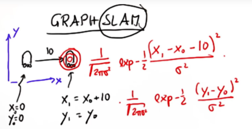
What Graph SLAM does is define our probabilities using the above constraints.
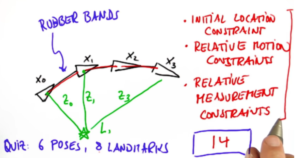
Consider the following Illustration. Suppose we have a robot that moves in a 2-dimensional space. Each location is characterized by a vector x0,x1, etc. x0 is our intial location constraint. Each movement has a relative motion constraint given by the gaussians above. These movements can be seen as rubber bands so to speak. In a perfect world the actual motion will equal the commanded motion, but in reality it might have to bend a bit. Since we're building a map we take measurements $Z_0,Z_1,Z_2$ to some landmark $L_1$.
Quiz: 6 poses, 8 Landmarks equals how many constraints?
Ans: 14. 1 Initial localization + 5 relative motion constraints + 8 relative measurement
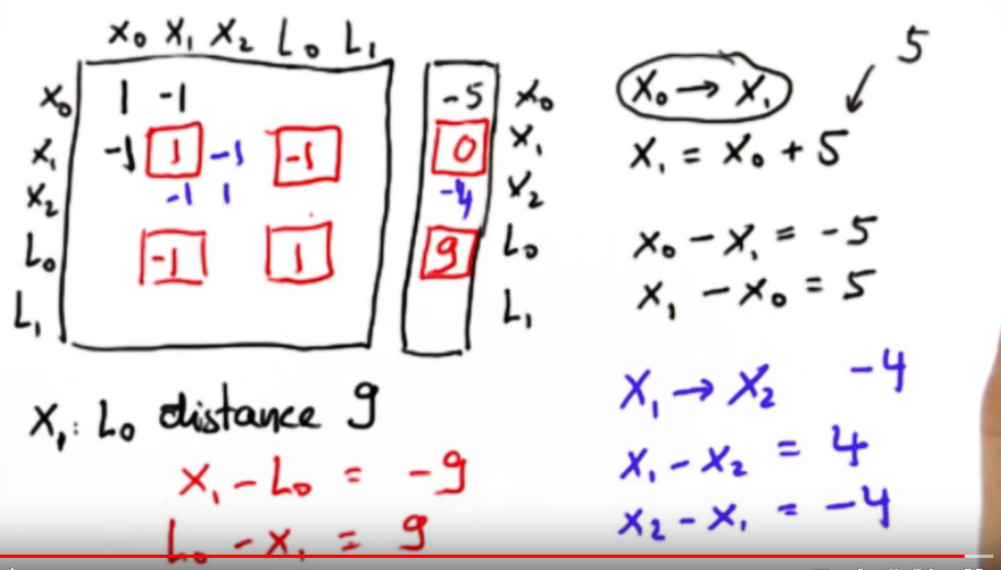
To implement this we simply create a matrix and a vector that represents our linear system of constraints. This can be a bit tricky to build. Suppose moving from $X_0->X_1$ is 5 then we write $X_1 - X_0 = 5$ and $X_0 - X_1 = -5$. Similarly if X1 to X2 is -4 then $X_1-X_2=4$ and $X_2-X_1=-4$. Now we incorporate the second pair of equations into our matrix to get $-1*X_0+2*X_1+-1*X_2 = 9$. We continue this iterative approach to build our matrix.
The next step will be to incorporate the distances to our Landmarks L_0 and L_1.
Suppose we begin with the belief that L0 is a distance of 9 from X1.
Hence $x_1 - L_0 = -9$ so we subtract 9 from the $X_1$ element of the vector
and $L_0 - X_1 = 9$ meaning we
- a. add 1 to element (r4,c4)
- b. add -1 to elements (r2,c2), (r4,c2)
- c. add 9 to L0 element in the vector
When we integrate this into the matrix we get the following.
Finally we need to integrate the initial robot location constraint.
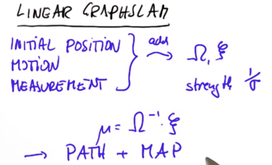
We can solve this system for the best possible estimates $\mu$ as $\Omega^{-1} + \xi$.
Here's a more fullsome example
Given X0=-3, X1=X0+5, X2=X1+3. You should get mu = [-3, 2, 5]
We construct our omega matrix as
   X0  X1  X2   Xi
X0  2  -1   0   -8
X1 -1   1  -1    2
X2  0  -1   1    3
One can also perform this programmatically as follows
Omega = [[1,0,0],[0,0,0],[0,0,0]]
Xi = [[init],[0],[0]]

#This time we add to the first
Omega += [[1,-1,0],[-1,1,0],[0,0,0]]
Xi += [[-move1],[move1],[0]]

Omega += [[0,0,0],[0,1,-1],[0,-1,1]]
Xi += [[0],[-move2],[move2]]

mu = Inverse(Omega) dot Xi
Now to extend this to include Landmark columns
# We expand Omega from 3x3 to 4x4, and copy over the original
Omega = Omega.expand(4,4,[0,1,2],[0,1,2])
# We expand Xi from 3x1 to 4x1, and copy over the original
Xi = Xi.expand(4,1,[0,1,2],[0])
# Set the X0,L0 measurement Z0
Omega += [[1,0,0,-1],[0,0,0,0],[0,0,0,0],[-1,0,0,1]]
Xi += [[-Z0],[0],[0],[Z0]]
# Set the X1,L0 measurement Z1
Omega += [[0,0,0,0],[0,1,0,-1],[0,0,0,0],[0,-1,0,1]]
Xi += [[0],[-Z1],[0],[Z1]]
# Set the X2,L0 measurement Z2
Omega += [[0,0,0,0],[0,0,0,0],[0,0,1,-1],[0,0,-1,1]]
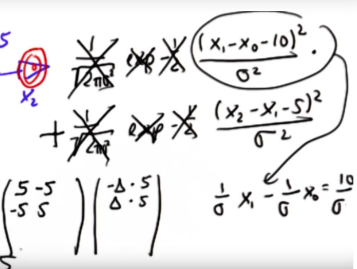
Xi += [[0],[0],[-Z2],[Z2]]If you recall when we began we looked at the initial constraint of x,y as the product of 2 gaussians. It turns out that you don't even need to complicate things. If you replace a product with a sum, and just keep the exponential term then you get a similar equation to that found in the omega matrix. This time however, the x terms have a coefficient in terms of 1/sigma. This tells us to regulate, or weight, a measurement higher we simply need to increase the coefficients in Omega.
To summarize
Weakness
The matrix Omega and vector C grow linearly with the length of the path, even though the map is of a fixed size. Hence the larger the matrix the slower the algorithm gets. There is a way to combat this by only keeping the most recent position x.
Consider the matrix Omega where the first col & row corresponds to X_t, the rest of the cols and rows correspond to the landmark observations. When we get a new movement X_t+1 we expand omega and insert X_t+1 into the 2nd row and column. Initially we simply set X_t+1 to a row of zero's. We then apply our motion update similar to before, this increases our path.
In order to reduce we solve for
Omega = Omega' - A.T B.inverse A
Xi = Xi' - A.T B.inverse C

Extra A-GraphSLAM
- Use a graph to represent the problem
- Each node in the graph corresponds to a pose of the robot during mapping
- Each edge between nodes corresponds to a spatial constraint between them
Graph Based SLAM build the graph and find a node configuration that minimize the error introduced by the constraints.