Machine Learning for trading¶

0 - Intro¶

Syllabus http://lucylabs.gatech.edu/ml4t/

Youtube Videos https://www.youtube.com/watch?v=s5xKxliBMTo&list=PLAwxTw4SYaPnIRwl6rad_mYwEk4Gmj7Mx

The course is divided into 3 main areas:

Manipulating financial data with python
Computational investing
Learning algorithms for trading

Three textbooks are used

Python for finance
What hedge funds really do
Machine Learning by Tom Mitchell

Without further adieu - Let's get started

1 - Python for Finance¶

1.1 Play with your data¶

Manual approach ( As of May2021 )

Investing.com will provide historical data.
Marketwatch also provides historical data, but is limited to 1 year

I've decided to download URTY, UDOW, and SPY for May-01-2020 to May-21-2021

Now we just load into pandas. Assuming you

import pandas as pd
# It's easier to format the dates when reading 
df = pd.read_csv("CS7646_resources/URTY.csv", parse_dates=['Date'])
# show first 5 rows
#df.head()
# show last n rows
df.tail(4)

We leave it to the reader to try out the following commands

df.columns              # get your columns 
df.dtypes               # get each columns datatype
df.iloc[5]              # get row 6 index = 5
print (df[10:21])       # print rows between index 10 and 20 inclusive
df['Price'].max()       # compute and return max
df['Volume'].mean()     # Compute Mean Volume

# Plotting for the very first time can be tricky 
# so we provide an example
import pandas as pd
import matplotlib.pyplot as plt
%matplotlib inline

df = pd.read_csv("CS7646_resources/URTY.csv")
# tailor to suit your ideal chart size 
#                                [width, height]
plt.rcParams['figure.figsize'] = [20, 5]
# Just one plot
#df['Price'].plot()

# plt.show()  # must be called to show plots
# If running from a python script 
#    remove       %matplotlib inline
#       add       plt.show()           at bottom
# want to see multiple columns plotted?
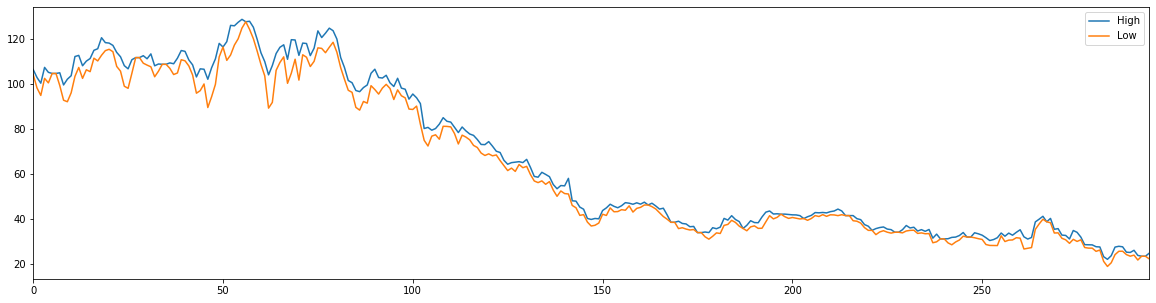
df[['High','Low']].plot()

<matplotlib.axes._subplots.AxesSubplot at 0x180130d9888>

1.2 Multiple stocks & Slicing¶

So far we've looked at only one stock. What if we want multiple stocks in one dataframe? Our data has the exact same dates, but this is NOT an accurate reflection of the real world.

Dataframes can be created in a multitude of ways

# from a dictionary
d = {'col1': [1, 2], 'col2': [3, 4]}
df = pd.DataFrame(data=d)
# from an array
df2 = pd.DataFrame(np.array([[1, 2, 3], [4, 5, 6], [7, 8, 9]]), columns=['a', 'b', 'c'])
# from a list of lists
data = [['tom', 10], ['nick', 15], ['juli', 14]]
df = pd.DataFrame(data, columns = ['Name', 'Age'])
# from a pair of dates
start_date,end_date = '2021-01-01', '2021-01-26'
dates=pd.date_range(start_date,end_date)
df1=pd.DataFrame(index=dates)

Of course 1 dataframe is rarely enough and we will need to join them

df1=df1.join(df2)               # Very basic join uses index as the key, and uses the default left join 
df1=df1.join(df2,how='inner')   # Very basic join uses index as the key, with a specified inner join 
# WARNING - columns names must be unique, otherwise you'll get an overlap error
# when performing a left join you may need to drop the na's
#      for example when there's no data
df1=df.dropna(subset=["Price"])

Now we get fancy

# Create 6 days
dates = pd.date_range("20130101", periods=6)
# dataframe indexed by dates, populated with random numbers
df = pd.DataFrame(np.random.randn(6, 4), index=dates, columns=list("ABCD"))

# Randomness with different datatypes
df2 = pd.DataFrame(
            {   "A": 1.0,
                "B": pd.Timestamp("20130102"),
                "C": pd.Series(1, index=list(range(4)), dtype="float32"),
                "D": np.array([3] * 4, dtype="int32"),
                "E": pd.Categorical(["test", "train", "test", "train"]),
                "F": "foo",
            }
        )

You can go so far as to convert to a numpy array as well.
df.to_numpy()
It should be noted however that this can be very expensive computationally. Reason being that a data frame data types are defined by each column. Whereas in numpy an array must be homogenous

import pandas as pd

start_date,end_date = '2021-01-01', '2021-01-26'
dates=pd.date_range(start_date,end_date)
df1=pd.DataFrame(index=dates)  # define empty dataframe with these dates as index

dfURTY = pd.read_csv("CS7646_resources/URTY.csv", 
                    index_col="Date", parse_dates=True, 
                    usecols=['Date','Price'], na_values=['nan'])

dfSPY = pd.read_csv("CS7646_resources/SPY.csv", 
                    index_col="Date", parse_dates=True, 
                    usecols=['Date','Price'], na_values=['nan'])

dfUDOW = pd.read_csv("CS7646_resources/UDOW.csv", 
                    index_col="Date", parse_dates=True, 
                    usecols=['Date','Price'], na_values=['nan'])

df1=df1.join(dfURTY)
df1.rename(columns={'Price': 'urty'}, inplace=True)

# default join is 'left', but you can specify
# df1 = df1.join(dfSPY, how='inner')
df1=df1.join(dfURTY)
# Rename column 
df1.rename(columns={'Price': 'spy'}, inplace=True)
df1=df1.join(dfURTY)
df1.rename(columns={'Price': 'udow'}, inplace=True)

df1.sort_index(axis=0,ascending=False,inplace=True)
# or you can use 
#            df1.sort_values(by='COLUMN_NAME')
# but this doesn't apply to the index column which has no name
df1.head()

More Selecting/Slicing

# You must sort first if you want to select based on date values
df_urty.sort_index(inplace=True)

# simple index slicing
df_urty[:3, 1:3]

# Using the index value 
print(df_urty.loc["20210501":"20210510"])

# Select a particular date
# Make sure the date you're looking for exists!!
dates = pd.date_range("20210401", periods=1)
df_urty.loc[dates[0]]
# Multiple Columns
df_urty.loc[dates[0],['Open','High','Low']]

# or use iloc with the indices
# Don't forget it includes the start index but not the ending
df_urty.iloc[1:3,2:4]
df_urty.iloc[1:3,[1,3]]
# Access a single value for a row/column pair by integer position.
df_urty.iat[3,3]
# Access a single value for a row/column label pair
df_urty.at["20200505",'Price']

Using Boolean Conditions

df_urty[df_urty['Price'] > 23.5]

# is in collections
df2["E"] = ["one", "one", "two", "three", "four", "three"]
df2[df2["E"].isin(["two", "four"])]

1.3 Power of Numpy¶

Mostly just a review of how to use numpy.
Here's a link Numpy Quick start

1.4 Pandas Stats and Feature Engineering¶

# Max & Min are similar to numpy
df_urty['Price'].max()
df_urty['Price'].min()

# computes for all numerical columns
df_urty.mean()             
df_urty.std()

"""Computing Rolling Statistics"""
# Compute rolling mean using a 20-day window
rm_SPY = df['SPY'].rolling( window=20).mean()

"""Computing Daily Returns"""
# The numpy way
# daily_returns[1:] = (df[1:] / df[:-1].values) - 1 # compute daily returns for row 1 onwards
daily_returns = (df / df.shift(1)) - 1 # much easier with Pandas!
daily_returns.iloc[0, :] = 0 # Pandas leaves the 0th row full of Nans

"""Computing Cumulative Returns"""
# Left to the reader :)
# Hint -> CumReturn[t] = (Price[t]/Price[0]) - 1

"""Bollinger Bands = (rollingMean+2StdDev,rollingMean-2StdDev) """
def get_bollinger_bands(rm, rstd):
    """Return upper and lower Bollinger Bands.
    Input : rm = pandas series containing a rolling mean
            rstd = pandas series containing a rolling standard deviation
    returns 2 pandas series
        upper_band = rolling mean + 2*rolling standard deviation
        lower_band = rolling mean - 2*rolling standard deviation
    """
    # Quiz: Compute upper_band and lower_band
    upper_band = rm + rstd * 2
    lower_band = rm - rstd * 2
    return upper_band, lower_band

1.5 Incomplete data¶

Rarely will we get complete data that is ready to use as is. Sometimes stocks don't trade and missing data will appear.

# to Identify missing values
missing = pd.isna(df["Price"])
# OR
df2.isna()

# HANDLING
# One common technique is to fill empty entries
df2.fillna(0)   # Replace NA with a scalar value
df2["one"].fillna("missing")

# You can fill forwards and backwards
df.fillna(method="pad")     # pad  / ffill    -- Fill Forward
df.fillna(method="bfill")   # bfill/ backfill -- Fill Backwards

# There is also shortcut functions
df.ffill()
df.bfill()
# Note that if you need to do both ALWAYS perform forwards first

# The last method we demostrate is interlpolate
df.interpolate()
# There are several methods available for Interpolate
df.interpolate(method="time")       # Index aware interpolation (Index is dates)
df.interpolate(method="values")     # Index aware interpolation (Index is floating point)

import scipy as sp
df.interpolate(method="quadratic")          # For a growing time series
df.interpolate(method="pchip")              # approximating values that are part of a cumulative distribution function
df.interpolate(method="akima")              # For smooth plotting
df.interpolate(method="spline",order=2)
df.interpolate(method="polynomial",order=2)

1.6 Histograms and Scatter Plots¶

# as usual - clean your data
# https://stackoverflow.com/questions/42135409/removing-a-character-from-entire-data-frame
df_urty.rename(columns={'Change %': 'Return'}, inplace=True)
df_urty['Return'] = df_urty['Return'].replace({'%':''}, regex=True).astype('float64')
returns = df_urty['Return']
# plotting a Histogram
# Plot a histogram
%matplotlib inline
returns.hist(bins=15,figsize=(20,5))  # changing no. of bins to 20
# If you get messy results check your input

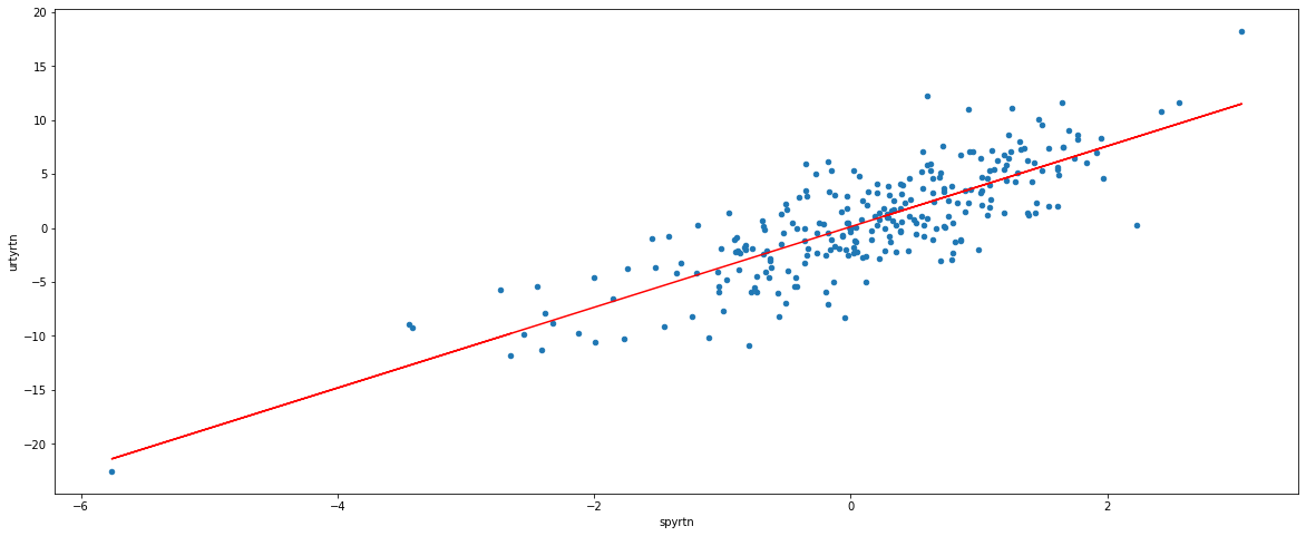
In this next section we take a look at the correlation between two stocks, urty & spy. We define beta as the slope of line measuring the relationship between a stock and the index spy. We define alpha as the interesction of the line with the y-axis

WARNING Beta is the slope of dependence. It is NOT a measure of correlation

import pandas as pd
import numpy as np
import matplotlib.pyplot as plt

df_urty = pd.read_csv("CS7646_resources/URTY.csv", 
                    index_col="Date", parse_dates=True, 
                    na_values=['nan'])
df_urty.rename(columns={'Change %': 'urtyrtn'}, inplace=True)
df_urty['urtyrtn'] = df_urty['urtyrtn'].replace({'%':''}, regex=True).astype('float64')

df_spy = pd.read_csv("CS7646_resources/SPY.csv", 
                    index_col="Date", parse_dates=True, 
                    na_values=['nan'])
df_spy.rename(columns={'Change %': 'spyrtn'}, inplace=True)
df_spy['spyrtn'] = df_spy['spyrtn'].replace({'%':''}, regex=True).astype('float64')

df = df_urty[['urtyrtn']].join(df_spy[['spyrtn']], how='inner')
#df.head()
df.plot(kind='scatter', x='spyrtn', y='urtyrtn', figsize=(20,8))
beta_urty, alpha_urty = np.polyfit(df['spyrtn'], df['urtyrtn'], deg=1)
# we choose deg=1 to imply a line of the form  
# y = bx + a 
print ("beta_urty= ", beta_urty)
print ("alpha_urty=", alpha_urty)
plt.plot(df['spyrtn'], beta_urty*df['spyrtn'] + alpha_urty, '-',color='r')

df_corr = df[['spyrtn','urtyrtn']]
print('\n Here we can see the correlation')
print(df_corr.corr(method='pearson'))

# https://stackoverflow.com/questions/42135409/removing-a-character-from-entire-data-frame
# df[cols_to_check] = df[cols_to_check].replace({';':''}, regex=True)

#df_urty.tail()

beta_urty=  3.7341631386993104
alpha_urty= 0.11440514980575896

 Here we can see the correlation
           spyrtn   urtyrtn
spyrtn   1.000000  0.811719
urtyrtn  0.811719  1.000000

1.7 Sharpe Ratio¶

Pretty trivial formula:

portfolio_start_val = 1000000
start_date = 2009-1-1
end_date = 2011-12-31
symbols = ['SPY', 'XOM', 'GOOG', 'GLD']
allocations = [0.4, 0.4, 0.1, 0.1]


normed = prices/prices[0]
allocated = normed * allocations
pos_vals = allocated * portfolio_start_val
port_val = pos_vals.sum(axis=1)

daily_rets = daily_rets[1:]
cum_ret = (port_val[-1]/port_val[0] - 1)
avg_daily_ret = daily_rets.mean()
std_daily_ret = daily_rets.std()

k = 252  # of samples per year (NOT the number of samples)
         # ie if using daily data then k = 252 = number of business days in 1 year 
         # ie if using weekly data then k = 52 = number of weeks in 1 year 
daily_rf = 0.0
SharpeRatio = sqrt(k) * mean(daily_rets - daily_rf) / std(daily_rets)

NB: technically we should subtract std(daily_rf) from the denominator. But this is often a constant and is therefore dropped.

risk free rate options/estimators:

LIBOR - London InterBank Offer Rate: which is the borrowing cost between banks
3mth T-Bill (treasury bill)
or just 0

1.8 Optimizers: Building a parameterized model¶

Note Bene This section requires the use of scipy.optimize

An optimizer is simply an algorithm to

find minimum values
build a parametrized model (polynomial fit)
refine allocation to stock portfolio

Using an optimizer boils down to three parts:

define a function to minimize
provide an initial guess
call the optimizer

Example:
Minimize a scalar function of one or more variables using Sequential Least Squares Programming (SLSQP).

import scipy.optimize as spo

def f(X):
    return (X - 1.5)**2 + 0.5
Xguess = 0   # random guess to use as a starting pt  
min_result = spo.minimize(f, Xguess, method='SLSQP', options={'disp': True})

If you run the above you will get the below results
Notice the value of x at the final line. This is the minimum

Optimization terminated successfully.    (Exit mode 0)
            Current function value: 0.5
            Iterations: 2
            Function evaluations: 7
            Gradient evaluations: 2
     fun: 0.5
     jac: array([1.49011612e-08])
 message: 'Optimization terminated successfully.'
    nfev: 7
     nit: 2
    njev: 2
  status: 0
 success: True
       x: array([1.5])

Optimizers will have difficulties when a function is not convex. Wikipedia-Convex function
Recall that a function f(x) is convex iff the line segment for any two points on a graph lie above the graph.

In other words: if we draw a line between any two points on the graph, then all points on the graph must be below the line. If at any point inbetween the line endpoints is above the line then there will be more than 1 minimum.

Convex

import scipy.optimize as spo

def f(X):
    return (X - 1.5)**2 + 0.5

Xguess = 0
# Minimize a scalar function of one or more variables using Sequential Least Squares Programming (SLSQP).
min_result = spo.minimize(f, Xguess, method='SLSQP', options={'disp': True})
print(min_result)

Optimization terminated successfully.    (Exit mode 0)
            Current function value: 0.5
            Iterations: 2
            Function evaluations: 7
            Gradient evaluations: 2
     fun: 0.5
     jac: array([1.49011612e-08])
 message: 'Optimization terminated successfully.'
    nfev: 7
     nit: 2
    njev: 2
  status: 0
 success: True
       x: array([1.5])

Building a Parametrized Model

This next example demonstrates fitting a line using an optimizer

import numpy as np
import scipy.optimize as spo

# random line : slope and intercept
l_orig = np.float32([4, 2])

# data construction based on our line
Xorig = np.linspace(0, 10, 100)
Yorig = l_orig[0] * Xorig + l_orig[1]

# Generate noisy data points => Data + noise
noise_sigma = 3.0
noise = np.random.normal(0, noise_sigma, Yorig.shape)
data = np.asarray([Xorig, Yorig + noise]).T
# Uncomment to see plot
# plt.plot(data[:,0], data[:, 1], 'go', label="Data points")

# Try to fit a line to this data
# we will use a sum of square error minimization approach
def error_func(line, data): 
    #            actualvalue -  estimated value 
    return np.sum((data[:,1] - (line[0] * data[:, 0] + line[1])) ** 2)

# Generate initial guess for line model 
l = np.float32([0, np.mean(data[:, 1])])  # slope = 0, intercept = mean(y values)

# Call optimizer to minimize error function
result = spo.minimize(error_func, l, args=(data,), method = 'SLSQP', options={'disp': True})
print(result)

Optimization terminated successfully.    (Exit mode 0)
            Current function value: 888.7485857375983
            Iterations: 3
            Function evaluations: 18
            Gradient evaluations: 3
     fun: 888.7485857375983
     jac: array([0.00439453, 0.00059509])
 message: 'Optimization terminated successfully.'
    nfev: 18
     nit: 3
    njev: 3
  status: 0
 success: True
       x: array([4.13022838, 1.10273294])

"""Minimize an objective function using SciPy: 3D"""

import pandas as pd
import matplotlib.pyplot as plt
import numpy as np
import scipy.optimize as spo

def error_poly(C, data): # error function
    """
    Compute error between given polynomial and observed data.
    Inputs
        C   : numpy.poly1d object or equivalent array representing polynomial coefficients
        data: 2D array where each row is a point (x, y)
    Outputs
        err (int) = error as a single real value.
    """
    # Metric: Sum of squared Y-axis differences
    err = np.sum((data[:,1] - np.polyval(C, data[:,0])) ** 2)
    return err

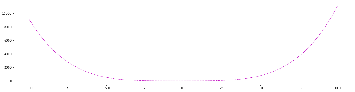
def fit_poly(data, error_func, degree=3):
    """Fit a polynomial to given data, using a supplied error function.

    Parameters
    ----------
    data: 2D array where each row is a point (X0, Y)
    error_func: function that computes the error between a polynomial and observed data

    Returns polynomial that minimizes the error function.
    """
    # Generate initial guess for line model (all coeffs = 1)
    Cguess = np.poly1d(np.ones(degree + 1, dtype=np.float32))

    # Plot initial guess (optional)
    x = np.linspace(-5, 5, 21)
    plt.plot(x, np.polyval(Cguess, x), 'm--', linewidth=2.0, label = "Initial guess")

    # Call optimizer to minimize error function
    result = spo.minimize(error_func, Cguess, args=(data,), method = 'SLSQP', options={'disp': True})
    return np.poly1d(result.x) # convert optimal result into a poly1d object and return


def test_run():
    # Define original line a polynomial of degree 2
    l_orig = np.float32([1.5,-10, -5, 60, 50])
    t = (-10*(l_orig[0]**4)) + (-10*(l_orig[1]**3)) + (-10*l_orig[2]**2)+ (-10*l_orig[3]) + l_orig[4]
    print(t)
    # data construction based on our line
    Xorig = np.linspace(-10, 10, 100)
    # bad bad bad
    # the exponents belong to the xorig values. l_orig are the co-efficients
    # Yorig = (Xorig*(l_orig[0]**4)) + (Xorig*(l_orig[1]**3)) + (Xorig*l_orig[2]**2)+ (Xorig*l_orig[3]) + l_orig[4]
    Yorig = np.polyval(l_orig, Xorig)
    
    print(Xorig[0],Yorig[0])
    
    # Generate noisy data points => Data + noise
    noise_sigma = 1.0
    noise = np.random.normal(0, noise_sigma, Yorig.shape)
    data = np.asarray([Xorig, Yorig + noise]).T

    # Try to fit a line to this data
    # Generate initial guess for line model (all coeffs = 1)
    degree = 4
    Cguess = np.poly1d(np.ones(degree + 1, dtype=np.float32))
    
    # Plot initial guess (optional)
    x = np.linspace(-10, 10, 50)
    plt.rcParams['figure.figsize'] = [20, 5]
    plt.plot(x, np.polyval(Cguess, x), 'm--', linewidth=1.0, label = "Initial guess")
    
    
    # Call optimizer to minimize error function
    result = spo.minimize(error_poly, Cguess, args=(data,), method = 'SLSQP', options={'disp': True})
    final = np.poly1d(result.x)
    print(final) 
    
    
test_run()

9149.375
-10.0 23950.0
Optimization terminated successfully.    (Exit mode 0)
            Current function value: 103.24155966774836
            Iterations: 8
            Function evaluations: 84
            Gradient evaluations: 8
     4      3         2
1.5 x - 10 x - 4.998 x + 59.99 x + 50.08

Test - Portfolio Optimizer¶

3 Machine Learning basics¶

3.01 ML at Hedge funds¶

The ML problem: given x(observations) how can we determine y
Ex: Given price momentum, Bollinger Values how can we determine the future price?

Supervised regression learning:

Regression boils down to a numerical prediction.
Supervised means were are given some examples (inputs and outputs)
Learning means we train with data

Consider the problem of robot navigation. X would be the inputs coming from the sensors and Y would be the resulting direction change. If learning is introduced then it will use it's memory whenever it encounters previous situations.

Similarly for a stock we may have the history of a stock features, as well as the output price. The first step in building our model is constructing our data. Determining what features are important, determine the time period as well as possible determining any related stocks.

Once you've built a model you need to test it, this is called backtesting. Backtesting is where you run your model on past data to determine it's accuracy. While simple to explain this is not as simple as it appears. A model run on data used to build it is fraught with challenges. Regression models can be noisy and uncertain. It's also difficult to measure and estimate uncertainty.

3.02 Regression¶

This section is about Supervised Regression learning. where Regression is defined as a numerical model. Suppose your data consists of barometric and rainfall measurements. We want to be able to predict rainfall as a model of barometric measurement. The classical approach to this might be to fit a line $rain = barometer*x+b$ but there are other approaches. Another approach might be to take an input baramoter reading, then locate, or query the data, for the k-nearest neighbours and take their mean to estimate the output (rainfall).

Our examples so far have been rather simplistic and limited. As a problem grows in size, scope and ambiguity, the approach to modelling is different. Parametric models are used for problems limited in scope. For example a cannon ball distance based on angle is straight forward. But consider honey bee production relative to the richness of their food. Linear Regression would fall into the parametric approach because the model is known, it simply needs to be fitted. But in the honey bee case we would a nonparametric model such as K-means regression.

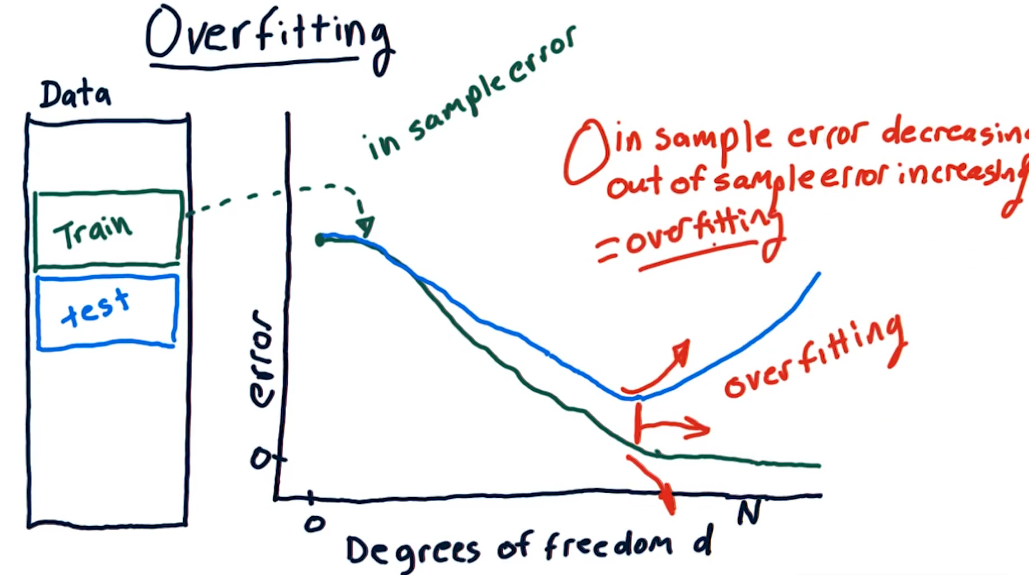
To build our model we begin by splitting our data into a train and test sets. Since we are dealing with time sensitive data our train data should always be the oldest, making the test data the most recent.

We will be implemented several learners to assess their quality on the problem of stock modelling.

Our models will follow a similar pattern:

Each model will be wrapped inside a class (LinRegLearner, KNNLearner)
Each class will have a train method that takes inputs and outputs belonging to the training data
Each class will need to have a query method that takes the test data

Example

class LinRegLearner:
    def __init__():
        pass
    # y = Mx+b
    def train(xtrain,ytrain):
        self.M, self.b = your_favourite_linreg()
    def query(X)
        y = self.M * X + self.b
        return y

class KNNLearner:
    # simply modify the above accordingly

3.03 Assessing Learning Algos¶

Recall our Knn Solution. We define our k for some constant, take some training data and create an algo from it. Suppose we take k=3 and we test our query. At different points the values used in the k algo will of course change. If we take k to an extreme, say equal to the number of points then we just end up with an average value over all points for any point we input to the model. Similarly if we take k as just 1 then for each input to the model only 1 value is returned, and that value is the corresponding value from the training data. In other words we have perfectly fit the model ... meaning we have overfit the model.

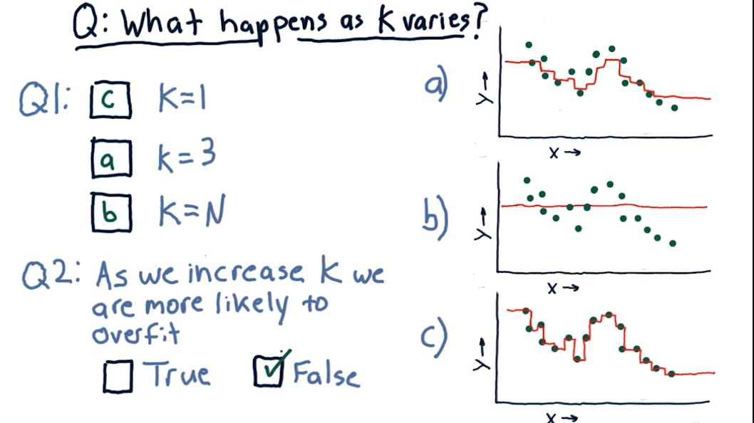
A similar phenomena occurs when fitting a parametric model of an arbitrary degree

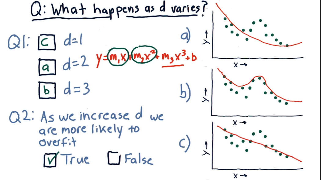
Of course visuals are nice and all but the truth is in the details. We want to quantify the above. RMS to the rescue. RMS is the Root Mean Square error. And is defined as follows.

$$RMS = \sqrt{ \frac{\sum(y_{test}-y_{predict})^2}{N} }$$

where y_predict is the result produced by our model, and y_test is the expected result as given by our test data.

Warning In most ML model building lifecycles we would perform a cross validation where we take random samples for our training and testing data. When dealing with a time series data it doesn't make sense. If you do include recent data into the training phase then you've effectively used the future data to build the model. This simply doesn't work.

What you can do is perform Roll Forward cross validation. This is where you're training data is always some time frame before your test data. After the first test you increment your time frame and test against the next set of data. This allows you to perform repeated train-test steps without peaking into the future.

Evaluate the accuracy by measuring the difference (RMS error) between the predicted results and the actual values. This is measured quantitatively by the correlation. NB correlation measures how well the line (aka model) fits the results. It is not the slope of the line. In general a large RMS error implies a low correlation.

What is overfitting? Suppose we wanted to graph the degrees of freedom d against our RMS error e. To help visualize this think of a polynomial with degree d. As the degree of freedom increases from 0 the error will decrease. BUT there will be a point where the error (against the test data) will resume increase, while the insample error (training data) continues to decrease

What if we repeated the same experiment using a Knn model? Well for k=1 it is clear that the error will be small but as k increases so does the error. If you recall for k=n, n=sample size, the model will return the average over all values.

3.04 Ensemble Learners: Bagging and boosting¶

Can weak learners be combined to create a single strong learner? It turns out YES! To learn how this done read on!

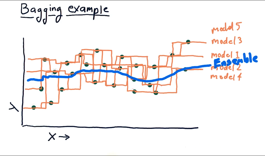
In the previous sections we looked at learners that produce a base model. In an ensemble model we combine these learners into a single model, how we combine can be multifaceted. In general ensemble learners have a lower error and are less likely to be overfitted. Ideally ensembles should combine models of different types, for example a knn and a polynomial.

Method 1 (Bootstrapping or bagging): In this method we train models based on different subsets of data. So we might choose n samples from our training subset and create a model from it. Then we could query each model and take the mean of each, to produce our result. Thus our result is driven by a ensemble of each model.

Boosting is very similar to bagging. The big difference here is that a weighting factor is introduced. Models with a higher error get a lower weight and will affect the results less. The most popular implementation of this is the adaBooster. It should be noted that boosting is prone to overfitting.

3.05 Decision Trees 1¶

2 Market Fundamentals¶

2.01 So you wanna be a hedge fund manager¶

How do funds work? Well first let's get some basic assumptions down first.

Every hedge fund, and fund manager, effectively manage a portfolio of stocks. This portfolio is a basket of stocks. The main types of funds are:

ETF : which is a fund of stocks and is traded on a stock exchange and are highly transparent
Mutual Funds : Less transparent and less liquid. Bought and sold at the end of each day, quarterly disclosures
Hedge funds : No transparency or disclosures, generally contractual, low liquidity and cannot be bought/sold without permission

A key topic for all fund managers is the compensation which is tied to the fund AUM (Assets under Management)

ETF managers often get an expense ratio of 0.01% to 1.00%
Mutual Fund managers get an expense ratio of 0.5% to 3.00%
Hedge fund managers often get "two & twenty" meaning 2% of the AUM plus 20% of the profits

Example : Two and Twenty
You manage a fund which started the year at 100M and grew to 115M by year end.
So you'll get 2% of 100M (2M) and 20% of the 15M profit (3M). You just made 5M for the year

Expense ratio and the 2 and 20 approach both motivate the manager differently

Both approaches will motivate AUM accumulation, since both will increase as AUM increases.
2/20 incentivizes profits
2/20 incentivizes risk taking

Hedge Funds attract large institutions, funds of funds, and very wealthy individuals. In order to sell themselves there are a few approaches. A track record spanning 5 or more years, a good simulation and story, portfolio fit (do you fill an area they haven't already covered)

Sharpe Ratio Also known as the risk adjusted return (see section 1.07)

Fundamentally a hedge fund will calculate a "Target Portfolio" that it wants to achieve. Of course it would also have a "Live Portfolio" which it is trying to push as close as possible to the target. To do this it has an algorithm that is analyzing market data to determine the next best step.

All of these elements are highly dependent on the approach taken. An algo can analyze realtime tick (order data), or live price data, or both of course.

2.02 Market Mechanics¶

There are many online brokers that will execute your order. This section deals with how your order is fulfilled.

First What is an order?

Action (buy or sell)
Symbol - ie what are you ordering
Quantity: the size of your order
Type: Limit or market, how flexible are you
Price: relative to the type, will place a constraint on the order

Second The order book
This is where the exchange places your order. Highly anonymous and publicly available. Often reveals interest in an symbol. Each order will be segmented into two main types: Asks and Bids. Ask is for selling, bids are to buy. (recall that exchanges are essentially auctions). Price movement can be approximated using these orders. High number of asks and low number of bids will pressure the price towards the bid price.

Caveat: with so few exchanges and so many investors orders may often be executed at a Dark Pool. A quasi exchange often managed by a few brokers which can relieve pressure on an exchange.

How Hedge Funds exploit market Mechanics Imagine you are in seattle and make an order that goes to a pool in atlanta. The hedge fund sits in NY and has very low latency, especially considering your distance. HF monitors the order book and observes that the price is going up, so it buys. You hit buy at the same time as well. BUT you are far away! So the HF order is received and filled by the exchange well ahead of you. This could be just a second ahead of you but a second could mean thousands of orders at an exchange. So now the hedge fund in newer york turns around and put a sell order in at a price higher than it bought. Your order will now be filled at the new sell price. All of this takes place in a few milliseconds which makes a world of difference.

A similar situation will also occur whenever your dealing with a large distance. London vs NYSE can contain a discrepancy for a few milliseconds. The HF orders in fact help to equalize these prices very rapidly

Exchanges Handle: Buy, Sell, Market Limit
Brokers Handle Stop loss, Stop gain, Trailing stop, sell short.

Short Selling Used when the price is expected to go down.
You think xyz is going to decrease in price. So you borrow xyz from someone and you turnaround and sell it. Example: 100 xyz is borrowed at a price of \$100.00 pershare, for a total value of \\$10,000.00, and you promptly sell it. After 1 month the price is \$90/share so you buy 100share (total \\$9000) and you prompty pay off your lender. You've just made 1000 dollars in 1 month.

Of course life isn't always so simple. The risk in short selling is when your wrong, ie when the price goes up contrary to your expectations. There is no limit to how high a stock price can go, what this means is there is no limit to the potential loss or risk in short selling. When you buy your risk is limited to the purchase price, but the reward is unlimited.

2.03 What is a Company Worth¶

Suppose you have a company that makes \$1.00 per year. What is this company worth? There's many ways of looking at value. The most likely possible choice would be say 10-50 dollars depending on Interest rates. The reason for this is based on some basic assumptions. Suppose you have 70 years left in your life then you could expect to make \\$70.00. But since the value of a dollar today is higher than a dollar in 1 year we need to discount these future dollars.

A company has three types of values. A true value, an Intrinsic value, and a Market Value. Market Value is the easiest and determined by the market price of it's stock multiplied by the shares outstanding. The Intrinsic value is the present value of the future returns. Book Value reflects the value of the companies assets, in other words it's balance sheet of it's assets. Book value includes things like inventory, but not something like future returns.

Present Value of Money
A dollar now is worth more than a dollar tomorrow. How do we express this mathematically? $$ PV = \frac{FV}{(1+i)^p}$$
Where FV is the future value, i is the interest/risk rate and p is the number of coumpounding periods.

The interest rate is called by many names depending on the context. The risk rate, interest rate, return rate are just a few. It also tells you a lot about the asset. For example government bonds will have relatively low return rates when compared to say a corporate bond dividend rate.

Intrinsic Value The present value of all future dividends
Here we alter the above equation and use the discount rate (dr).
$$ IntrinsicValue = PV = \frac{FV}{dr}$$ For example our company that pays \$1.00 per year would be worth \\$20.00 at a discount rate of 5%.

Book Value Total assets minus intangible assets and liabilities.
Suppose a company has 4 factories worth 10M apiece. It also has 3 patents worth 15M. and a 10M loan
Then the Company book value is 40M - 10M = 30M. Patents are ignored since they're considered intangible.

Market Value Shares outstanding x Market Price

The power of information: Ever notice how news affects stock price? The reason for this is simple: it affects the value that is computed by the above equations. Suppose the factories in the last example are in an area where war broke out. Would their value remain 10M apiece. Probably not.

2.04 CAPM: Capital Asset Pricing Model¶

Definition

Portfolio is a weighted set of assets, we use $w_i$ to represent the weights and their absolute values should sum to 1. NB a negative weight implies a shorted stock
Return of a portfolio is defined as $r_p(t) = \sum_i w_i r_i(t)$

Consider 2 assets A & B, with weights 75% and -25%, and the returns for 1 day are +1% and -2% respectively.
What's the return for the portfolio?

75% of 1% is .75%; -25% implies that the stock was shorted, so (-25%)*-2% yields .50%
Our total 1 day return is thus 1.25%

The Market Portfolio
In each country there is a index that is widely considered as representative of their market or economy. Some examples are

USA it is S&P500,
UK it is the FTSE
Japan it is the TOPIX, or potentially the Nikkei

These indices are composed of many stocks, and are generally Cap weighted. Meaning their weight is capped $w_i = \frac{MarketCap_i}{\sum MCaps} $. And these indices can often be broken down even further into various sectors.

The CAPM Equation $ r_i(t) = \beta_i r_m(t) + \alpha_i(t) $ where $r_m$ is the market return
To fully understand notice what this says notice that

$r_i$ is dependent on $r_m$ which has a significant effect
$\beta_i$ is a market relationship factor, and is the slope of the asset vs market plot
$\alpha_i$ is the residual with an expected value of 0

Active v Passive Management

passive: Buy an index and hold
active: pick stocks with various weight allocations

w.r.t CAPm both types of management will treat Beta and $r_m$ similarly but $\alpha$ is a different story. According to CAPm alpha should be random with an expected value of 0. Passive managers agree with this. However active managers do not, they take the position that alpha can be predicted in some form. For example alpha is positive for a stock that will go up, and vice versa. They may not always be right but on average they believe they are.

CAPM for Portfolios Can be easily derived from the original
$r_p(t)=\sum w_i (\beta_i r_m(t) + \alpha_i(t))$
$r_p(t)=\beta_p r_m(t) + \alpha_p(t))$ ( where $\beta_p = \sum_i w_i \beta_i$ )
or
$r_p(t)=\beta_p r_m(t) + \sum w_i \alpha_i(t))$ under active management

Implications of CAPM : In upwards markets you want a larger beta, but in downwards markets you want a smaller beta.

APT : Pricing Theory You can get a more accurate beta by breaking it out into it's individual sector component.

2.05 How hedge funds use CAPM¶

Typical Hedge funds look for stocks that perform well relative to the market. ie stocks that rise faster than the market and fall slower than the market.

Consider:
StockA prediction is 1% over market (w beta of 1.0) So they take a long position of \$50.00 StockA prediction is -1% below market (w beta of 2.0) So they take a short position of -\\$50.00

Scenario 1 : Time frame of 10days, Market is 0% after 10 days, our prediction is true
Then we get a return from A of 1% of 50 (0.50) + return from B of -1% of -50 (0.50). Our final result is \$1.00 = 1%

Scenario 2 : Time frame of 10 days, Market is +10\% after 10days, then
$r_A = (1.0)*10% + 1% = 11% => (50*11%)=5.50$
$r_B =-1*( (2.0)*10% + -1%) = -19% => (50*-19%)=-9.50$ (Note that we multiply by -1 to represent our short position!)
Total return : -\$4.00 which is Return rate : -4%

Scenario 3 : Time frame of 10 days, Market is -\10% after 10days, then
$r_A = (1.0)*-10% + 1% = -9% => (50*-9%)=-4.50$
$r_B =-1*( (2.0)*-10% + -1%) = 21% => (50*21%)=10.50$ Total return \$6.00 with a return rate of 12\%

What have we learned? Well if you don't position your position properly you can still lose.

In reality though what often happens is that funds use the expected value of the CAPM over the portfolio under multiple scenarios

\begin{equation} \begin{split} r_p & = \sum_i w_i (\beta_i r_m + \alpha_i) \\ & = (w_A \beta_A + w_B \beta_B ) r_m + (w_A \alpha_A + w_B \alpha_B ) \\ & = (0.5*1 + -0.5*2.0) r_m + (0.5*1 + -0.5*-1.0) \\ & = -0.5*r_m + 1.0 \end{split} \end{equation}

Now we have an equation that can equalize the expected value. A followup quastion might be how do we eliminate the market risk? ie we want $(w_A \beta_A + w_B \beta_B ) = 0$

This is just a linear optimization problem. We want weights $w_A$ and $w_B$ such that $\beta_p = 1*w_A + 2.0*w_B = 0$ we can express this as $w_A = -2*w_B$ since B is shorted. You may also recall that $w_A + w_B =0$ by definition of the weights of a portfolio. So
$w_A = -2*w_B$ and $abs(w_A)+abs(w_B)=1$
Now sub 1 into 2 to get $abs(-2*w_B)+abs(w_B)=1$
Which we can solve to get $abs(w_B)=\frac{1}{3}$ and simplify to get the final solution
$w_B=\frac{-1}{3}$ and $w_A=-2*w_B=\frac{2}{3}$

So what's the point of all this? Well we've shown how to eliminate the market risk. If we use the above to construct our portfolio then we will make a 1\% return in either a good or a bad market.

All that is left is to find stocks with a good alpha! Alpha is also often thought of as information. News about a company is also information.

2.06 Technical Analysis¶

There are two broad approaches to determining value: Fundamental vs Technical Analysis. Fundamental analysis uses metrics that are reflected on the company's balance sheet. Technical analysis focuses on the the price and volume only. Technical analysis uses these two features to build indicators or heuristics that they believe are indicative of future returns. While controversial in many circles they borrow heavily from statistical analysis.

Technical analysis is most effective when:

combinations of individual indicators are used (weaker as the number of indicators nears 1)
Looking for contrasts (ie stock vs market)
Shorter time periods (the trading horizon)

NB: The longer the trading horizon the more you should lean towards fundamental analysis.

A few popular indicators are:

Momentum: the price change over a rolling fixed period of time (Price(t)/Price(t-n) - 1)
simple moving average: the average price over a fixed, but rolling, window of time
- To quantify this is often used as a ratio of the price
- (Price[t]/Price[t-n:t].mean()) - 1
Bollinger Bands: comes from an observation by Bollinger of volatility on price
- He proposed using bands of +2 and -2 sigma applied to the simple moving average
- One possible strategy is to sell when the price goes over sma+2sigma
- similarly buy when price goes below sma-2sigma
- otherwise we just hold it

Often time when indicators are applied to a raw price they can potentially overwhelm other indicators. In order to give them a fair treatment we normalize so that each indicator will be between -1 and 1

Normed = ( Values - Mean ) / Standard deviation

2.07 Dealing with Data¶

Data Aggregation There are many Exchanges with their own order books. At the lowest granular level data is represented as Ticks. A tick is a successfull buy/sell match or transaction. These happen independent of time, although they do have a time stamp, and of course different exchanges may have different ticks in the same time span. These will be consolidated into periodic chunks (minute/hour/day etc). The close is the last transaction in the periodic chunk.

Handling Stock Splits
You may notice that in some days the price of a stock drops or jumps significantly. Significant meaning far outside the normal range of deviation. This is usually the result of a stock split.

Here's an example:
On monday Stock A is trading at \$300.00, and a 4:1 stock split is executed at the end of the day. On tuesday Stock A will open at \\$75.00, which is 300/4, also the number of outstanding shares will increase by 4

Clearly this will cause issues in our data. Left unhandled an algo might think that there was a drop.

We handle this by computing the "adjusted close". This is done by dividing the price by 4, for the data before the split. Pretty simple really. Notice that the price in the most recent data will always be the same as the adjusted close, since the most recent data will be after a split

Also notice that a reverse split is the opposite. A company might perform a 1:4 reverse split. In this case you're 4 shares become 1. Consequently the price is now 4 x Presplit price.

Handling Dividends
Many companys pay a dividend that is often reflected in the price of a stock. Upon payment the stock will almost always drop the exact same amount.

Here's an example:
On monday Stock A is trading at \$100.00, and will pay \\$1.00 in dividend per share at the end of day.
On Tuesday what do expect the share price to be? \$99.00 of course. There is another consideration when dealing with dividends. They're announced well before they are paid, their announcement will trigger a gradual price rise so that on the payment date the announced divident is priced into the market price.

Handling dividends follows the same pattern as a split. Compute the dividend as a percent, then decrease, or discount, the actual historical prices by that percentage to get the adjusted close.

Similar to splits the adjusted remains the same as the market price for dates after the dividend payment, but will diverge more and more the further back in history you go.

Survivor Bias
When developing a strategy you should aim to use survivor bias free data. This means that company's that have disappeared from the exchange are present in the historical data. A good case in point is the S&P 500. If you were to look at it today and pull the stocks you would not see the 50+ company that went bankrupt due to the 2008 financial crisis. If you built a strategy on today's S&P data it would be totally ignorant to the potential of financial distress. As you can imagine this is certainly a large gap in the development of a strategy.

2.08 EMH: Efficient Market Hypothesis¶

Although we haven't explicitly stated it we have been using, and operating, under multiple assumptions

There are a large number of investors
New information arrives randomly
prices adjust quickly
prices reflect all available information

Where does info come from?

Price and volume (public, rapid, quick)
Fundamental data (public, periodic)
Exogenous - Public info external to the company (ie oil prices to an airline)
Company insiders (least accessible)

Three forms, or versions, of the EMH

Weak: Future prices cannot be predicted from historical prices
- prohibits tech analysis
- Allows for fundamental info
SemiStrong: Prices adjust rapidly to new public info
- prohibits both tech and fundamental info
- allows for company insider info
Strong: Price reflect all information both public and private
- excludes tech, fundamental and insider info

2.09 Fundamental Law of Active Portfolio Management¶

The importance of diversification!

Developed by Richard Grinold and Ronald Kahn, the Fundamental Law of Active Management states that an active manager’s productivity depends on the quality of his/her skills and, consequently, the frequency in which the skills are applied at work. The law can also be expressed in an equation. The active manager should produce the Information Ratio (IR), which is the added value in every unit of risk added.

Grinold's Fundamental law: the relation between Skill, Performance, and breadth.
$Performance = skill * \sqrt{breadth}$
$IR = IC * \sqrt{BR}$
where

IR = Information Ratio, similar to the sharpe ratio of excess returns (in excess of the market return)
IC = the skill level
BR = Breadth = the number of trading opportunities

Example:
Coin flipping experiment : We bet on heads, or tails, of a flip instead of a stock. The coin is biased - like $\alpha$ 0.51 of getting heads, Uncertainty is like $\beta$

Betting: We bet N coins: Win - get 2N coins, Lose - now have 0
Environment: 1000 tables, 1000 tokens, games run in parallel

3 options

A1 bet all 1000 tokens on a single table
A2 bet 1 token on each of the tables
A3 doesn't matter? they're equivalent

Method 1 : Expected Return

A1: (0.51 x 1000) + (0.49 x 1000) = \$20.00
A2: 1000 x (0.51 x 1 + 0.49 x 1) = \$20.00

From the above it might appear that they are equivalent. What isn't apparent here is the risk or variance.

We might ask what is the probability we lose it all? Under A1 there is a .49 chance we lose it all. Under A2 the probability is (0.49^1000) ... which is incredibly small

Method 2 : Standard deviation

Under A2 => stdev(-1,1,-1,1,-1,-1,-1,...) = 1.0
Under A1 => stdev(1000,0,0,0,0,...) = 31.62

Method 3 : Reward/Risk

A1 : \$20.00/\\$31.62 = 0.63
A2 : \$20.00/\\$1.00 = \$20.00

It is interesting to note as well that $20.00 = 0.63 x \sqrt{1000}$

What does this all tell us?

Higher alpha generates a higher sharpe ratio
More execution opportunities provides a higher sharpe ratio
sharpe ratio grows as the square root of breadth

IR: Information Ratio
Recall that Portfolio return under CAPM $r_p(t)=\beta_p r_m(t)+\alpha_p(t)$
Suppose we wanted to compute the sharpe ratio of the skill component $\alpha_p(t)$
Then $IR = \frac{mean(\alpha_p(t))}{stdev(\alpha_p(t))} = \frac{Reward}{Risk}$
IR is often thought of as the sharpe of excess returns

IC: Information Coefficient: Is the correlation of forecasts to returns

BR: Breadth: Is the number of trading opportunties per year

$IR = IC x \sqrt{BR}$ = Performance = Skill x square_root(Breadth) What this means is that opportunities are needed. You can improve your performance by improving your skill or improving your breadth. In general improving your opportunties is much easier!!

Consider a real world case:
Warren Buffet holds 120 stocks, Simons of Rentech hedge fund holds thousands of stocks. Both have the same IR, but Simon's hedge fund algo has an IC of 1/1000 of Buffet's

How many trades must simon execute? (ANS: 120,000,000)
Why?
$IC_b \sqrt{120} = IC_s \sqrt{x}$
$IC_b \sqrt{120} = \frac{1}{1000} \sqrt{x}$
$IC_b \sqrt{120} = \frac{IC_b}{1000} \sqrt{x}$
$1000 \sqrt{120} = \sqrt{x}$
$1000^2 120 = x$
$x = 120,000,000$

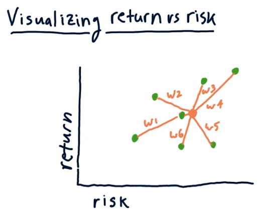
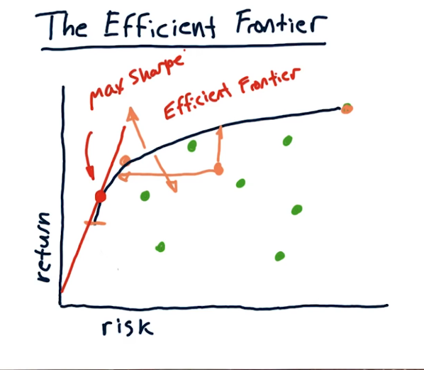
2.10 Portfolio Optimization and Efficient Frontier¶

Suppose you have a set of stocks you think are promising. How much of your portfolio should you invest in each? This is the question that portfolio optimization, aka Mean variance optimization, seeks to answer.

ie Given a set of equities and a target return, find an allocation to each equity that minimizes risk.

Let's pause to consider what is risk? For us we define this as the standard deviation of historical daily returns. We can visualize this relation by graphing multiple stocks on a 2 dimensional plane. Each green dot represents the return and the risk of a given entity. The orange/brown dot represents a possible scenario for some abitrary weights. This would represent the risk and return of the portfolio with the respective weights.

Can we do better than this? In fact we can! As per Harry Markowitz we can minimize risk while increasing the returns.

Consider 3 stocks: A,B, and C each with a return of 10%. Furthermore suppose A and B are positively correlated with a covariance of 0.9, meaning they move in a similar fashion. Suppose A and C are negatively correlated with a covariance of -0.9.

Sc1: 50% A and 50% B will yield 10% but will not reduce volatility Sc2:.25A, .25B, and .5C will yield 10% but the volatility will be less than any one of the equities. This tells us that blending negatively correlated stocks is a great way to reduce volatility

Mean Variance Optimization (MVO):
Inputs: Expected Return, Volatility, Covariance, Target Return ( must be between max and min equity returns )
Outputs: Asset weights for portfolio that minimize risk

The Efficient Frontier:
For any return level there is an optimal portfolio.

4 Reinforcement Learning¶

4.01 Intro to RL¶

Until now we've focused on learners that provide a forecast. We've ignored the probability of the forecast.

Think of a robot in an some sensory environment, ie it has sensors for observation. This environment is what we call a state. It must then process this to formulate a policy, ie what it should do in such a state, this is generally denoted by pi $\pi(s)$. Once it processes the environment and determines a state then it must take action. This results in a new state. After all it's sensors will now yield new information. The cycle now repeats.

How is this policy determined? Well in an RL world each action results in a reward. For example if it's goal is to reach a point then each action that results in a distance closer to the goal is a positive reward.

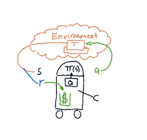
How do we map the world of trading to fit an RL Problem?

Actions: Buy, Sell, Hold, etc
States : Holding Long or short, Technical indicator values
Reward : Return from exiting a trade

Daily return can be thought of either a reward or even a state.

Markov Decision Problem
RL problems solve and MDP defined in terms of

a set of states S
a set of actions A
A transition function T[s,a,s]
and a Reward Function R[s,a]

The Goal: Is to find $\pi(s)$ that will maximize the reward. and we denote this as $\pi^*(s)$

We often don't know T nor do we know we know R. But what we can do is build and record our experiences as a series of tuples. for example
$<s_1,a_1,s'_1, r_1>, $
$<s_2,a_2,s'_2, r_2>, $ here $s_2=s'_1$ from previous row
... $<s_n,a_n,s'_n, r_n>, $

We do this over and over to gain experience. Now we can build T by accumulating the first three elements into a matrix, or some other tabular representation. Similarly we can accumulate, build R. Then we use Value/Policy iteration approach to build our policy and try to optimize.

Consider the following Problem.

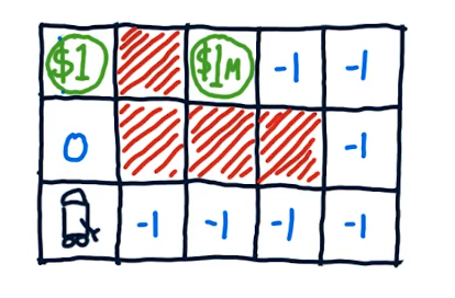
There's 2 possible rewards 1 and 1 million. the 1 will come back and be obtained multiple times, but the 1 million is a once time only reward. If we placed a constraint like giving the robot gas for only 3 moves then the best option is to go for the one. If we gave the robot up to 8 moves they should aim for the 1 million. Now recall our future dollar value from 2.01. A dollar now is worth more than one in the future.

We can summarize our three reward scenarios as follows

Infinite Horizon: $\sum_{i=1}^\infty r_i$
finite Horizon: $\sum_{i=1}^n r_i$
Discounted Reward: $\sum_{i=1}^\infty \lambda^{i-1} r_i$ this is what we use in Q-learning.

4.02 Q-Learning¶

Q-Learning is a model free approach, meaning it doesn't know about nor does it use transitions and rewards tables. What it does is it builds a table of utility(Q) values as it interacts with the world. Interestingly, it can be shown that Q learning is guaranteed to provide an optimal policy.

Q learning is named after the q function. Q can be thought of either as a function or a table, for our purposes we take the table approach. It has 2 dimensions (s,a) representing the state and action. Q represents the value of taking action a in state s. This is the immediate reward + the discounted reward.

Suppose we have a Q-Table, how do we use it? Well we simply take the best policy
ie $\pi(s) = argmax_a(Q[s,a])$
Now as we build this table and it gets larger and larger then we will converge to the optimal policy
ie $\pi^*(s) = Q^*[s,a]$

This doesn't tell us how we build our Q table. Here's a general algo

High Level

Select training and test data
Iterate over time <s,a,s',r>
Test policy $\pi$
Repeat until convergence

The key is the iteration in point #2 above which requires it's own algo

set the start time and initialize Q (This is often done with small random numbers)
compute s
select a
step forward and observe r & s'
- <s,a,s',r> now comes from these 3 points
update Q

Given <s,a,s',r> how do we improve the Q table?

Part 1: $Q'[s,a] = (1-\alpha)Q[s,a] + \alpha ImprovedEstimate $ where alpha is between 0 and 1 Part 2: $Q'[s,a] = (1-\alpha)Q[s,a] + \alpha ( r x \lambda later reward ) $ where lambda is between 0 and 1 which is $Q'[s,a] = (1-\alpha)Q[s,a] + \alpha ( r x \lambda Q[s',argmax_{a'}(Q[s',a'])$

Some Finer points:

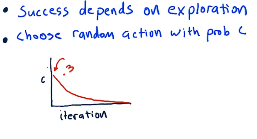
Success depends on exploration. We need to explore as much of the state and action space as possible. This is generally achieved through the use of randomness. For example at the start of our iteration we might choose a random action, this forces the system to explore actions it might not otherwise come across.

How do we translate this to Trading?

Actions are straight forward. We have Buy, Sell, and hold.
Rewards are a bit more nuanced. Using daily returns provides fast convergence, when compared to say cumulative returns. The reason for this is because the daily return is an immediate reward vs cumulative which is a delayed reward.

We need to represent our state as a single number. We will still with integers to keep things simple. To do this we Discretize and Combine. Discretization simply a mapping to an integer.

One simple method for discretizing into "steps"

stepsize = size(data)/steps
data.sort()
for i in range(0,step):
    threshold[i] = data[(i+1)*stepsize]

Summary: Building the model

define states, actions, rewards
choose in-sample training periods
iterate: Q-table update
backtest
repeat iteration+backtest until improvements cease

Test the model:

choose test periods

4.03 Dyna-QLearning¶

A significant shortcoming of Q-Learning is that it will take many experience tuples to achieve convergence. Dyna-Q enhances the Q-Learning by building a transition matrix T and a reward matrix R. After each interaction it will hullucinate hundreds or thousands of next scenarios which it thens uses to update the queue table.

Dyna-Q was developed by Richard Sutton. You'll recall that Q-Learning is model free, meaning it doesn't know T or Q.

Q-Learning algo is

init Q Table
Observe S
Execute a, Observe s and r
Update Q with <s,a,s',r>

Dyna-Q enhances it with the following steps

Learn T and R
- T'[s,a,s'] recall that this is the probability that taking action a from state s we will end up in s'
- R'[s,a] is the expected reward of taking action a in state s
Hallucinating experiences
- take s to be some random state s in our space S (call this s_rand)
- take a to be some random action a in our space A (call this a_rand)
- infer s' from T ( is what s' has the highest probability in the matrix T[s,a,?])
- determine r (r = R[s_rand,a_rand])
Update Q similar to before
Go back to 2 ( for some number of iterations, usually 1000s)

How do we learn T ? By observation of course. How many time does s and a lead to s', as a ratio to the number of times it doesn't. To perform this operation count the total number of trials and divide by the number that lead to s'

For example:

Initialize t_count = 0.0001 ( we can't use 0 because it may lead to division errors )
observe s,a,s'
increment T_count[s,a,s']

then we can evaluate T in terms of T_count: ie T[s,a,s'] = T_count[s,a,s'] / sum(T_count[s,a,:])

Learning R : $R'[s,a] = (1-\alpha)R[s,a] + \alpha * r $
Where

Alpha is our learning rate
R[s,a] is the expected reward of taking action a in state s
r is just our immediate reward

Verbally R is a weighted return favouring immediate rewards more than expected (future) returns

5 Derivatives¶

In this section we take a quick look at a particular type of Derivative securities called options. Options are contracts that confer a right to/on the buyer. This right is up to the buyer to exercise, meaning they also have the right, but not an obligation. The two main types of options are Calls and Puts.

5.01 Options¶

Defined:

Calls: Are the right to buy an asset at a fixed price ( ie Call for delivery )
Puts: Are the right to sell an asset at a fixed price ( ie Put up for delivery )

These options are part of a broader market class of instruments and securities called derivatives. In the market there will be buyers and sellers of each contract. The contracts for options consist of an asset that is generally 100 shares of an underlying stock, the fixed price is called the exercise, or strike, price.

There are many reasons why options exist:

Hedging: You own a stock and are worried it may go down, so you buy puts to guarantee a minimum price
- this can also be thought of as an insurance policy on your stock
Speculation: You think a stock will go up but don't want to tie up your money by buying the stock so you buy a call option
Make money: You own a stock you think is going up so you might write (aka sell) a put option to make a few extra bucks

Of course just as a stock is unpredicatable so are option prices difficult to pin point.

Example:
1 GM call option with a strike of \$50.00 is the right to buy 100 shares of GM for a price of \\$50.00 per share.

To complicate matters options also have an expiry date. Like most contracts it is only valid for a limited time. This makes sense as a buyer could hold an option in perpetuity.

Example:
Consider the following snapshot from Yahoo Finance taken July 31-2021, While AAPL trades for 145.86:

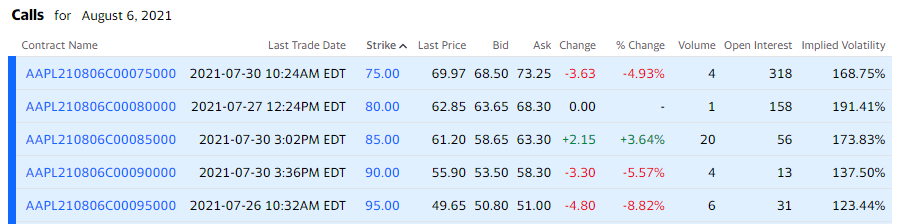
Suppose we buy AAPL calls on the 3rd row. What does this entail?

These Calls are for Aug 6 2021, meaning that is their expiration date. Afterwards they become worthless
The price for the third row is 61.20, this is a per share price. In other words the charge for buying this Call option would be 100 x 61.20 = \$6,120.00. Why so much?
Because AAPL is trading at 145.86 meaning each share is worth (145.86-85)=60.86. Notice how close this is to the price? That's not a coincidence. That slight difference is due to the volatility of the stock as well as the time remaining in the contract. There are 5 trading days left before it expires and it appears that the seller/market is expecting it to go up a few more dollars.

Let's now take a look at the profitability of these options.
Here we can see the profit loss curve for a Long call option.
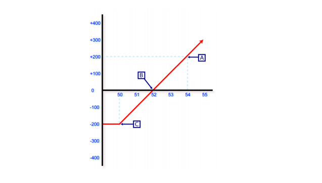We paid 200 for the option starting us in the red, this permium that we paid is our max loss. If the underlying stock goes to $52.00 we will break even meaning at 52 will gain 200 which will be offset by the premium/expense of 200. If the price of the underlying stock rises above 52, we will start to show a profit. In this case the profit is unlimited since it is a call on a underlying stock which do not have an upper limit on price.

For comparison here is a profit loss curve for a Long put option ( put with a strike at 50, and a premium of \$2.00 )
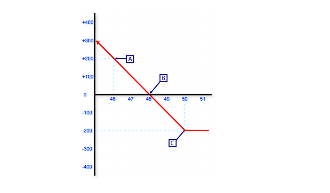Again we are limited in the amount of loss as well as profit. Missing from this graph is the left projection. Our profit reaches a max when the stock hits 0 dollars

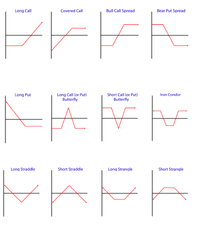
5.02 Options Strategies¶

Things get really interesting when you start building a portfolio with various combinations of options

Bull call uses two options with different strike prices
- Long call (strike > market) + Sell a call (strike > LongCall strike)
- used when betting that there will be a limited rise in price
- Limits the loss of owning the stock as well as capping the gain
Short call or put butterfly is a three part process
- Sell a put at s1 + buy a put at s2 < s1 + sell a put at s3 < s2
- Ex (Sell 105put at 6.25, +6.25)+(buy 2 100puts at 3.15, -6.30)+(sell 95put at 1.25, 1.45) = Net Credit/Gain is 1.20
- Both profit and loss will be capped
- Advanced strategy used in Bearish markets
- There is a small profit here so one should be careful of commision costs eroding this

A01 - Technical Trading Indicators¶

Stockcharts Technical Indicators

Investopedia

SMA - Simple Moving Average¶

Wikipedia

$SMA(k) = \frac{1}{k} \sum_{i=n-k+1}^n p(i)$

import pandas as pd
import numpy as np
product = {'month' : [1,2,3,4,5,6,7,8,9,10,11,12],'demand':[290,260,288,300,310,303,329,340,316,330,308,310]}
df = pd.DataFrame(product)

# 10 day simple moving average
df['LAG10SMA'] = df.iloc[:,1].rolling(window=10).mean()

EMA - Exponential Moving Average¶

Aka EWMA Exponential Weighted Moving average

$EMA(t) = (1-\alpha)EMA(t-1)+\alpha p(t)$

# 20 day EMA using Pandas 
#    adjust=False specifies that we are interested in the recursive calculation mode.
ema_short = data.ewm(span=20, adjust=False).mean()

MACD - Moving Average Convergence Divergence¶

Is a trend Following Momentum Indicator that shows the relationship between two moving averages of a securities price. It is calculated by subtracting the EMA(26day) from EMA(12day). ie ($EMA(12)-EMA(26)$)

Bollinger Bands¶

Composed of 3 lines to create 2 bands

Line 1 = SMA, generally used is a 20day sma
Line 2 = uBOL = SMA + 2 stdev
Line 3 = lBOL = SMA - 2 stdev

Notes

All computations should use the same period
numbers are typical and may be modified
Typical price can be used rather than close (Typical = High+low+Close / 3)

RSI - Relative Strength Index¶

https://school.stockcharts.com/doku.php?id=technical_indicators:relative_strength_index_rsi

$RSI = 100 - \left[ \frac{100}{1+RS} \right]$ where $RS=\frac{AvgGain}{AvgLoss}$

This is done in a 2 Part calculation Part 1 : For the first 14 days
Avg gain = sum of gains over the last 14 days / 14 Avg loss = sum of lossess over the last 14 days / 14

Part 2 : For subsequent days
Avg Gain = (PrevAvgGain x 13 + Current Gain ) / 14

#https://stackoverflow.com/questions/20526414/relative-strength-index-in-python-pandas
delta = price['Close'].diff()
dUp, dDown = delta.copy(), delta.copy()
dUp[dUp < 0] = 0
dDown[dDown > 0] = 0

RolUp = pd.rolling_mean(dUp, n)
RolDown = pd.rolling_mean(dDown, n).abs()

RS = RolUp / RolDown
rsi= 100.0 - (100.0 / (1.0 + RS))

# Alternatively using the EMA
## Make the positive gains (up) and negative gains (down) Series
#up, down = delta.clip(lower=0), delta.clip(upper=0)

## Calculate the EWMA
#roll_up = up.ewm(span=window_length).mean()
#roll_dn = down.abs().ewm(span=window_length).mean()

## Calculate the RSI based on EWMA
#RS = roll_up / roll_dn
#RSI = 100.0 - (100.0 / (1.0 + RS))

Money Flow Index¶

MoneyFlowIDX = 100 - ( 100 / (1 + MoneyFlowRatio))
Where
MoneyFlowRatio = 14Day_Positive_MoneyFlow / 14Day_Negative_MoneyFlow
RawMoneyFlow = Typical_Price x Volume
Typical_Price = (High + low + Close) / 3

Algo

Compute the typical price for each day
Compute the sign of the typical price wrt the previous day
Calc Raw Money Flow (Typical Price Volume sign)
Calc Money Flow Ratio
- Divide Raw Money flow into Positive and Negative flows
- add up the positive and divide by the sum of the negatives
Calc MoneyFlowIDX using the Money Flow Ratio

Volume Price Index¶

https://en.wikipedia.org/wiki/Volume%E2%80%93price_trend

A02 - Technical Trading Strategies¶

Moving Average Crossover¶

Inputs: A short and long moving average (can be of type EMA or SMA) BUY => when short MA moves above the long MA
SELL => when short MA moves below the longMA

Example: try 2 simple moving average with short=50day and long=200day

MACD Signal Crossover¶

Inputs: Signal Line = EMA(9day), MACD Line = (EMA12-EMA26) BUY => When MACD crosses the Signal from below, ie moves above the signal SELL => When MACD crosses the Signal from above, ie moves below the signal

	Date	Price	Open	High	Low	Vol.	Change %
291	2020-05-04	23.64	22.46	23.78	21.72	1.41M	1.03%
292	2020-05-03	23.40	23.40	23.40	23.40	-	0.00%
293	2020-05-02	23.40	23.40	23.40	23.40	-	0.00%
294	2020-05-01	23.40	24.57	24.76	22.23	2.92M	-11.83%

	urty	spy	udow
2021-01-26	100.11	100.11	100.11
2021-01-25	102.19	102.19	102.19
2021-01-24	NaN	NaN	NaN
2021-01-23	NaN	NaN	NaN
2021-01-22	102.53	102.53	102.53